Convolutional neural networks
About convolution
can be abstracted into mathematical expressions:

I can represent the matrix of an image, K is the convolution kernel
The computational layer of the convolution

Object Recogition with Gradient-Based Learning
- input layer Input Layer
- Convolution Layer Conv Layer
- Restricted Layer RELU Layer
- pooling layer Pooling Layer
- full connected layer
Creating a network Basic learning to distinguish between dogs and cats

(* Create model *)
myCatDogModel = NetChain[{
   ConvolutionLayer[32, 3], Ramp, PoolingLayer[2, 2],
   ConvolutionLayer[64, 3], Ramp, PoolingLayer[2, 2],
   FlattenLayer[],
   128,
   Ramp,
   2,
   SoftmaxLayer[]},
  "Input" -> NetEncoder[{"Image", {224, 224}, ColorSpace -> "RGB"}] ,
  "Output" -> NetDecoder[{"Class", {"cat", "dog"}}]]

(* Collect samples, training set and test set *)

(* Convert data sets to Association format *)
dataSetsConvert[dateSets_] := Module[
  {},
  File[#] -> StringSplit[FileBaseName[#], "."] [[1]] & /@ dateSets]
traingDataFiles = RandomSample[dataSetsConvert[traingData]];
testDataFiles = RandomSample[dataSetsConvert[testData]];

SetDirectory[
  "/Users/alexchen/datasets/Convolutional_Neural_Networks/dataset"];

FileNames["*.jpg", "training_set/cats/"];
FileNames["*.jpg", "training_set/dogs/"];
traingData =
  Join[FileNames["*.jpg", "training_set/cats/"],
   FileNames["*.jpg", "training_set/dogs/"]];
testData =
  Join[FileNames["*.jpg", "test_set/cats"],
   FileNames["*.jpg", "test_set/dogs"]];

(* Generate training and validation sets *)
traingDataFiles = RandomSample[dataSetsConvert[traingData]];
testDataFiles = RandomSample[dataSetsConvert[testData]];

(* sample is randomly selected for display *)
RandomSample[traingDataFiles, 5]

(* train the model *)
mytrainedModel =
 NetTrain[catdogModel, traingDataFiles, All,
  ValidationSet -> testDataFiles, MaxTrainingRounds -> 20]

(* Generate training model evaluation report *)
myModelPlot = mytrainedModel["FinalPlots"]

(* Generate the trained model to calculate the model correctness *)
myTrainedNet = mytrainedModel["TrainedNet"]
ClassifierMeasurements[myTrainedNet, testDataFiles, "Accuracy"]

Loss and error rate of the model

The final result obtained by ClassifierMeasurements[myTrainedNet, testDataFiles, “Accuracy”] is 75% i.e. the accuracy of the model is 75%
Under-fitting and over-fitting
From the above analysis, we can see that the orange line (learning of the training set) and the blue line (extrapolation of the validation set) are matching decreasing in the first five rounds of training, and in the later rounds, the model appears to be accurate for the training set, and the error rate increases instead of improving for the validation set, and the model appears to be overfitting.
The better the model fits the validation and training sets, the better the generalization ability of the model.

About convolution kernel KernelSize,Strid,PaddingSize
-
KernelSize: convolution kernel size e.g. 3 * 3
-
Strid: convolution kernel move step
-
PaddingSize: Convolution kernel boundary padding
-
Dilation: Dilation of the convolution kernel
The above parameters determine the dimensionality of the final output of our convolutional neural network

For example, in the model at the beginning, our input image is a RGB three-channel of size {128,128} i.e., tensor form {3,128,128}, after convolution kernelSize{3,3}, Stride{1,1}, Paddingsize{{0,0},{0,0}}, and Dilation{1,1}, we get This is because we set the PaddingSize boundary padding to {{0,0},{0,0}}, {{0,0},{0,0}} can be interpreted as {{xBegin,xEnd},{yBegin,yEnd}}, here the offset of x,y start and end is 0, the kernel will calculate the image size of {126,126}. When we add PaddingSize->{{1,1},{1,1}}, the size of the image after convolution kernel processing is the same as the original image, both are {128,128}.

About the dimension calculation of the output image of the convolution layer
Let the dimension of the input image be graph = {g1,g2,g3,… ,g(i)}, KernelSize = K, PaddingSize = {P_begin, P_end}, Strid = S, Dilation = Df, and compute the dimension of the output image as d = {d1,d2,d3,… ,d(i)}:
d(i) = (g(i) + P_begin + P_end - ((Df - 1) * (K - 1) + K))/S + 1 Result rounded
Simplify the equation as:
d(i) = (g(i) + P_begin + P_end - Df(K - 1) - 1)/S + 1 Result rounded
Based on the PaddingSize of {0,0} and {1,1}, we can calculate the output dimensions as {126,126} and {128,128}, respectively.
If ConvolutionLayer[64, 3, PaddingSize -> 1, “Stride” -> 2], i.e., the move step is 2, then according to the above formula we get the final dimensional output dimension as {64,64}, and the image is cropped to half of the original one, 3, PaddingSize -> 1, “Stride” -> 3], the image is cropped to {43,43}.
Also using the dilation parameter ConvolutionLayer[64, 3, PaddingSize -> 1, Dilation -> 2], we get the output image cropped to {126,126}, ConvolutionLayer[64, 3, PaddingSize -> 1, Dilation -> 3], the image is cropped to {124,124}.
About the dimensionality calculation of pooling layer
The pooling layer serves to reduce the dimensionality of the image, but retains important information.

MaxPoolinglayer parameters are:
-
Kernelsize: compute the kernel size
-
Stride: move step size
-
Paddingsize: the size of the boundary padding
The dimensional output of the pooling layer can be calculated in an analogous way to the output dimension of the convolutional layer.
Df = 1 for the pooling layer
d(i) = (g(i) + P_begin + P_end - K)/S + 1 The result is rounded
For example, if Paddingsize = {0,0}, kernelsize = {2,2}, and Stride S = {2,2}, then the computed output dimension is (128 + 0 + 0 - 2)/2 + 1 = 64, and if kernelsize = Stride = {3,3}, then Compute the output dimension as {42,42}.
Migration learning
Transfer learning is to freeze the characteristic layers on an already trained model and learn only the weight values of the last few layers to obtain a neural network that meets your needs.
Using VGG6 deep learning model
[VGG-16 Trained on ImageNet Competition Data](https://resources.wolframcloud.com/NeuralNetRepository/resources/VGG-16-Trained-on- ImageNet-Competition-Data)
vgg16Model = NetModel["VGG-16 Trained on ImageNet Competition Data"]
VGG16 contains a large number of convolutional layers, in order to filter and match features in the image

VGG16 can identify objects in 1000 images, currently we only need to identify dogs 🐶 and cats 🐱, so we need to modify the last few layers of the neural network.
Get the whole network up to the penultimate fourth layer 🙒 ðŸ™' tempNet = Take[NetModel[ “VGG-16 Trained on ImageNet Competition Data”], {1, -4}]
newNet = NetChain[<|“pretrainedNet” -> tempNet, “linearNew” -> LinearLayer[], “softmax” -> SoftmaxLayer[]|>, “Output” -> NetDecoder[{“Class”, {“cat”, “dog”}}]]
Train the model and freeze the weights of all layers except the linearNew layer
trainedNet = NetTrain[newNet, RandomSample[traingDataFiles, 1000], ValidationSet -> RandomSample[testDataFiles, 10], MaxTrainingRounds -> 3, LearningRateMultipliers -> {“linearNew” -> 1, _ -> 0}]
Finally, the correctness of migration learning is verified by randomly selecting 5 images from the validation set with 100% correctness

A randomly selected picture of a cat from the web is used to verify that the model's predictions are correct:

### The intermediate process of convolution layers ###
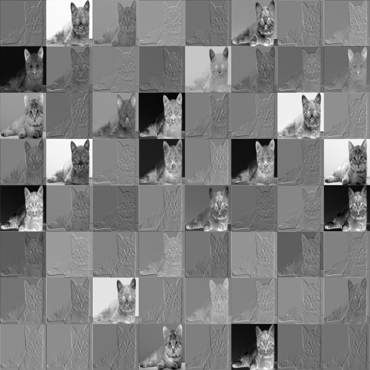
First get the feature output of the first convolutional layer conv1_1 (total 64 feature outputs):
convFeatures = trainedNet[🐱’s image,NetPort[{“pretrainedNet/conv1_1”, “Output”}]]; Dimensions[convFeatures] (* output: {64, 224, 224} *) ImageCollage[Map[ImageAdjust@*Image, convFeatures], ImageSize -> Medium]
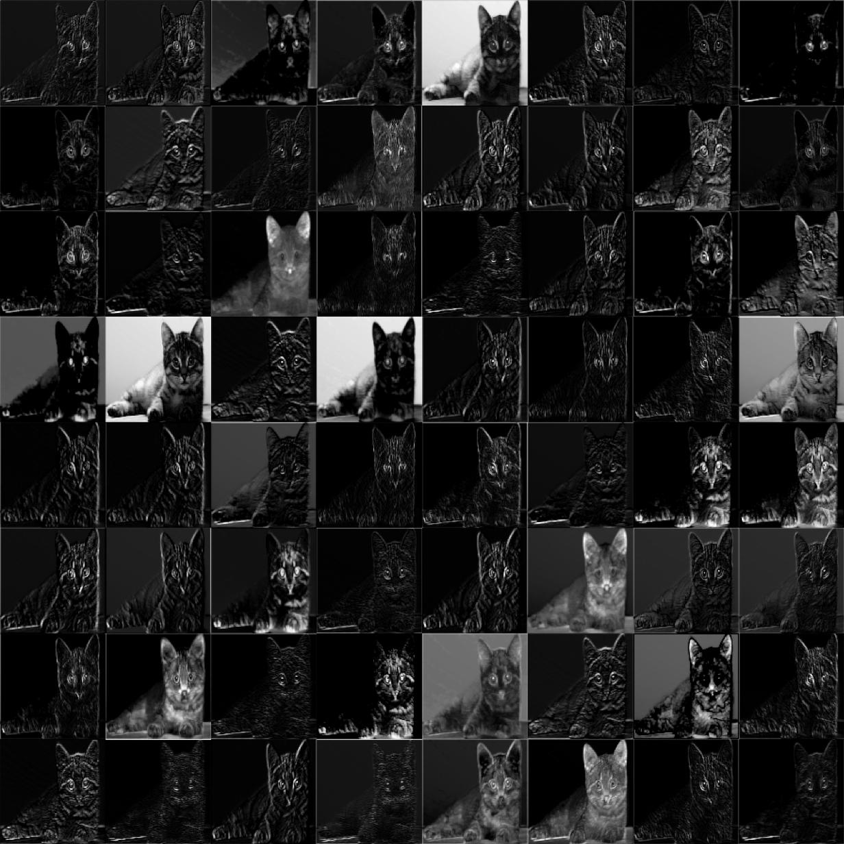
In the same way we can get the output image of the first pooling layer:
convFeatures = trainedNet[🐱’s image,NetPort[{“pretrainedNet/pool1”, “Output”}]]; Dimensions[convFeatures] (* output: {64, 112, 112} *) ImageCollage[Map[ImageAdjust@*Image, convFeatures], ImageSize -> Medium]
As can be seen, the pooling layer reduces the image dataset by half, but keeps the important information in it, which helps to reduce the consumption of computational resources during training.
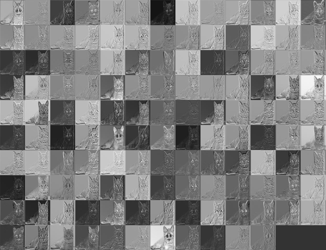
Get the output of pretrainedNet/conv2_1 features (128 features in total):
convFeatures = trainedNet[🐱’s image,NetPort[{“pretrainedNet/conv2_1”, “Output”}]]; Dimensions[convFeatures] (* output: {128, 112, 112} *) ImageCollage[Map[ImageAdjust@*Image, convFeatures], ImageSize -> Medium]
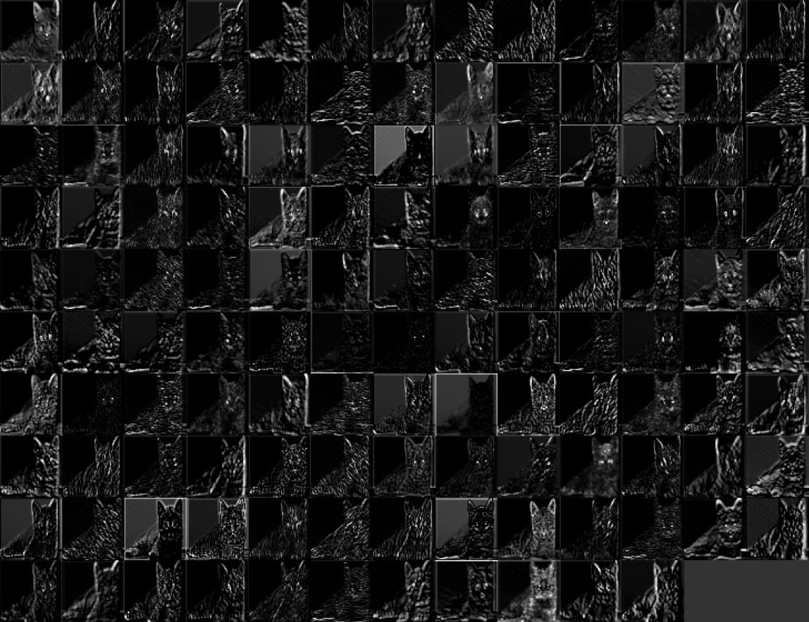
Output of the pooling layer:
And so on, we get the output of the third large layer of pretrainedNet-conv3_1 features (256 features in total)
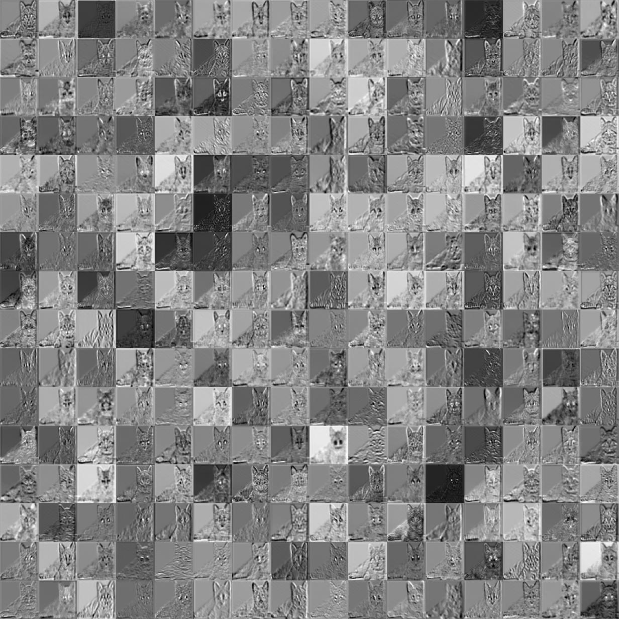
Output of the pooling layer:
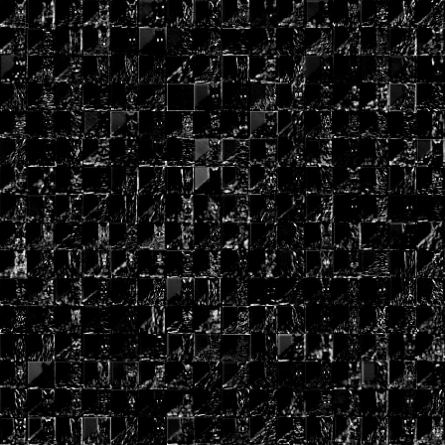
We can see that the convolutional neural network is continuously narrowing down the feature range, from the initial acquisition of the entire contour features of the cat to acquiring the edge contours such as the cat's ears, eyes, and nose, and then subdividing it into specific feature descriptions of the eyes and ears such as size, distance location information between them and other features, and finding edge detail features such as the nose, ears, and legs.
The fourth large layer of pretrainedNet/conv4_1 feature output (a total of 512 features)
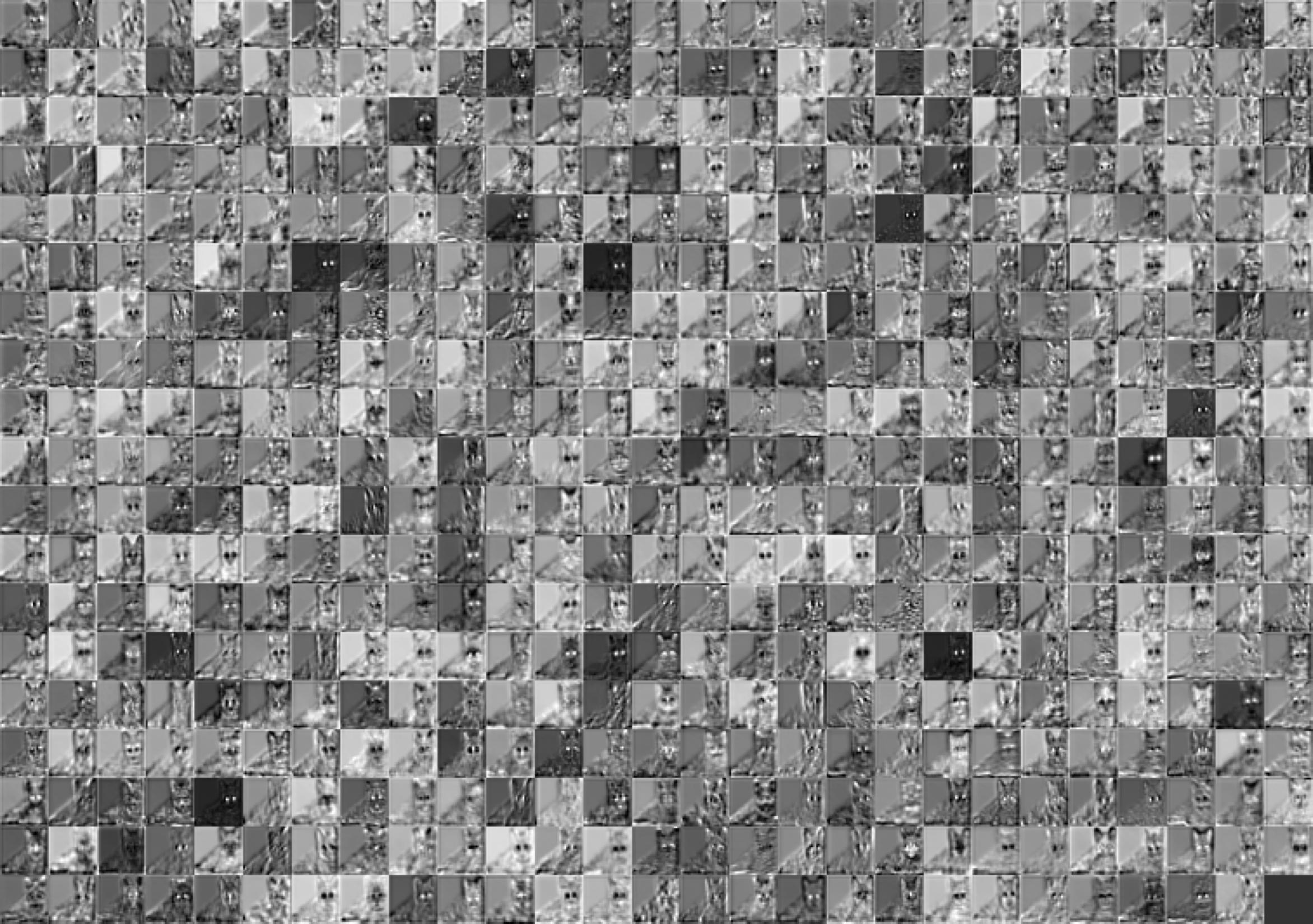
From this we can see that the neural network scans the whole image by convolutional kernels, the initial layer detects the edge contours of objects in the image, and then the higher the layer the more refined the features in the image, for example finding the cat's ears, the cat's eyes, the cat's mouth, and the cat's hair.
Each layer of the convolution kernel represents a feature representation :
weights = NetExtract[trainedNet, {“pretrainedNet/conv1_1”, “Weights”}]; ImageAdjust[Image[#, Interleaving -> False]] & /@ Normal[weights]
The visual representation of the convolution kernels for the first layer is as follows (64 convolution kernels in total):
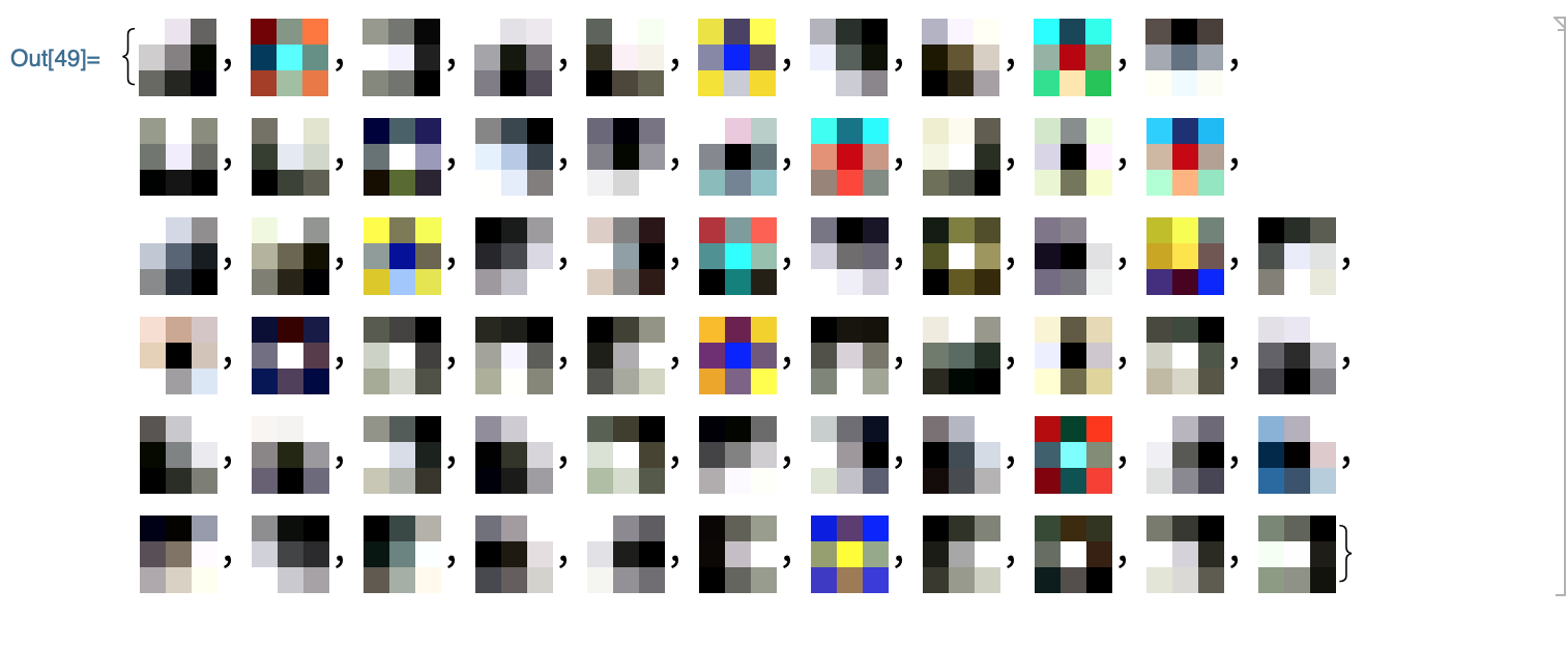
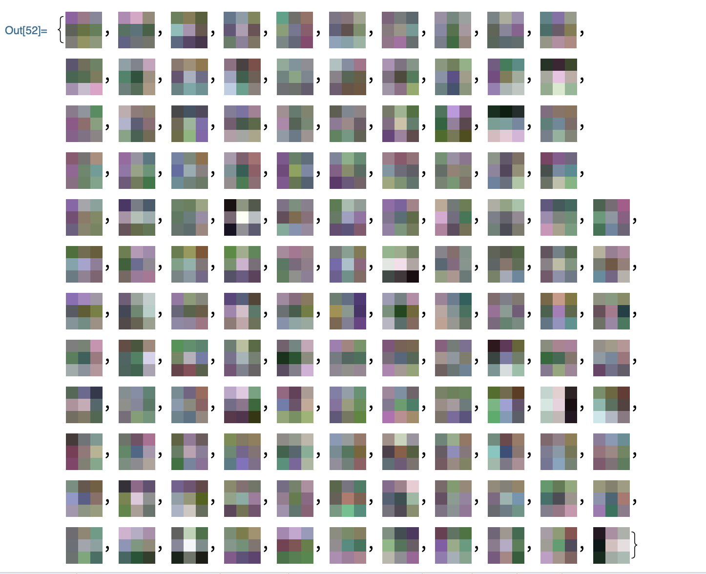
Visual representation of the second layer of convolution kernels:
### Algorithm ###
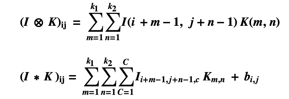
The forward computation of convolutional neural network is similar to that of artificial neural network. The following two expressions represent the forward computation expressions of convolutional network with channel number 1 and channel number C, respectively.
I denotes the image matrix, K denotes the convolution kernel, and for the convenience of corresponding to the conventional matrix, m,n iterates from 1. C represents the channels of the image, the number of channels of the grayscale image is 1, the number of channels of the image with color is 3, i.e. RGB three channels, and b represents the bias.
### Backpropagation of convolutional neural networks ###
The backpropagation of convolutional networks is also similar to the backpropagation of artificial neural networks, because the derivation of the backpropagation is more complicated, and it is likely that the wrong calculation is used in the derivation process, so this piece of algorithm derivation, I will independently put in DeepMind UCL course lesson 2 artificial neural networks and lesson 3 convolutional neural networks summary to rigorous derivation of these The back propagation of the two types of networks.
