History

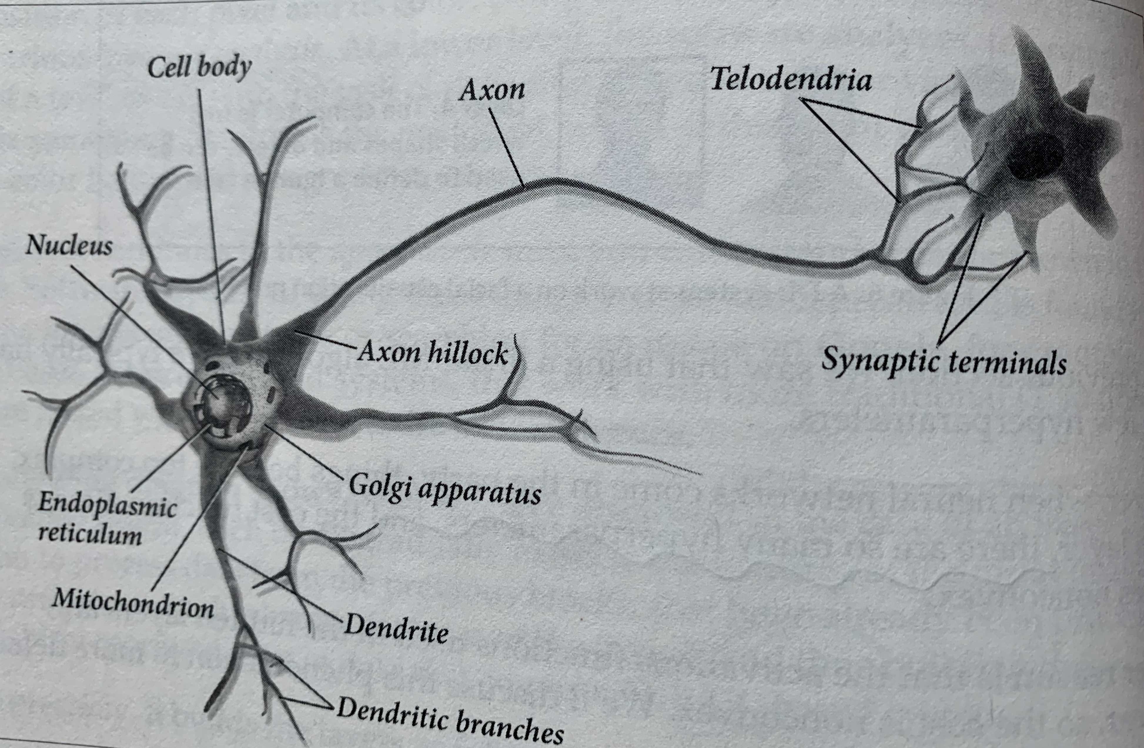
The original idea of developing neural networks came from the human study of the brain, which has a large number of biological neurons, as shown in the figure above. In the biological neuron model, electrical signals flow through the dendrite into the cell body, which is equivalent to a data processing center, and when there is enough stimulus response, it sends a weak electrical signal to the cable-like axon, which flows through the axon and then reaches the synaptic terminals. terminals), a neuron will have multiple dendrites and a single axon, and the signaling between neurons and neurons is accomplished through a conductive fluid in the synaptic gap. By modeling the biological neuron, an artificial neuron is obtained, and the four elements to build the corresponding model are as follows.

Biological model :

• Cell body
• axon
• Dendrites
• Synapse

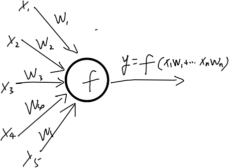
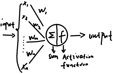
Artificial neuron:

• Cell body
• Output channels
• Input channels
• Weights

McCulloch and Pitts developed the first artificial neuron model based on biological neural networks. [Address of the paper A LOGICAL CALCULUS OF THE IDEAS IMMANENT IN NERVOUS ACTIVITY](https://www.cs.cmu.edu/~. /epxing/Class/10715/reading/McCulloch.and.Pitts.pdf)

Neuronal Models :

Machine learning

Deep learning is just a subset inside the set of machine learning, and the following is a general overview of machine learning in general.

Supervised learning

Algorithms:

• k-Nearest-Neighbors

• Linear Regression

• Logistic Regression

• Support Vector Machine

• Decision Trees

• Random Forests

• Neural networks

Unsupervised learning

Algorithms:

• Clustering

  • K-Means
  • DBSCAN
  • HCA (Hierarchical Cluster Analysis)

• Anomaly detection and novelty detection

  • One Class SVM
  • Isolation Forests

• Visualization Dimensionality reduction

  • PCA (principal component analysis)
  • Kernel PCA
  • Locally Linear Embedding (LLE)
  • t-distributed stochastic neighbor embedding (t-SNE)

• Association rule learning

  • Apriori
  • Eclat

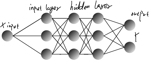
Neural network architecture

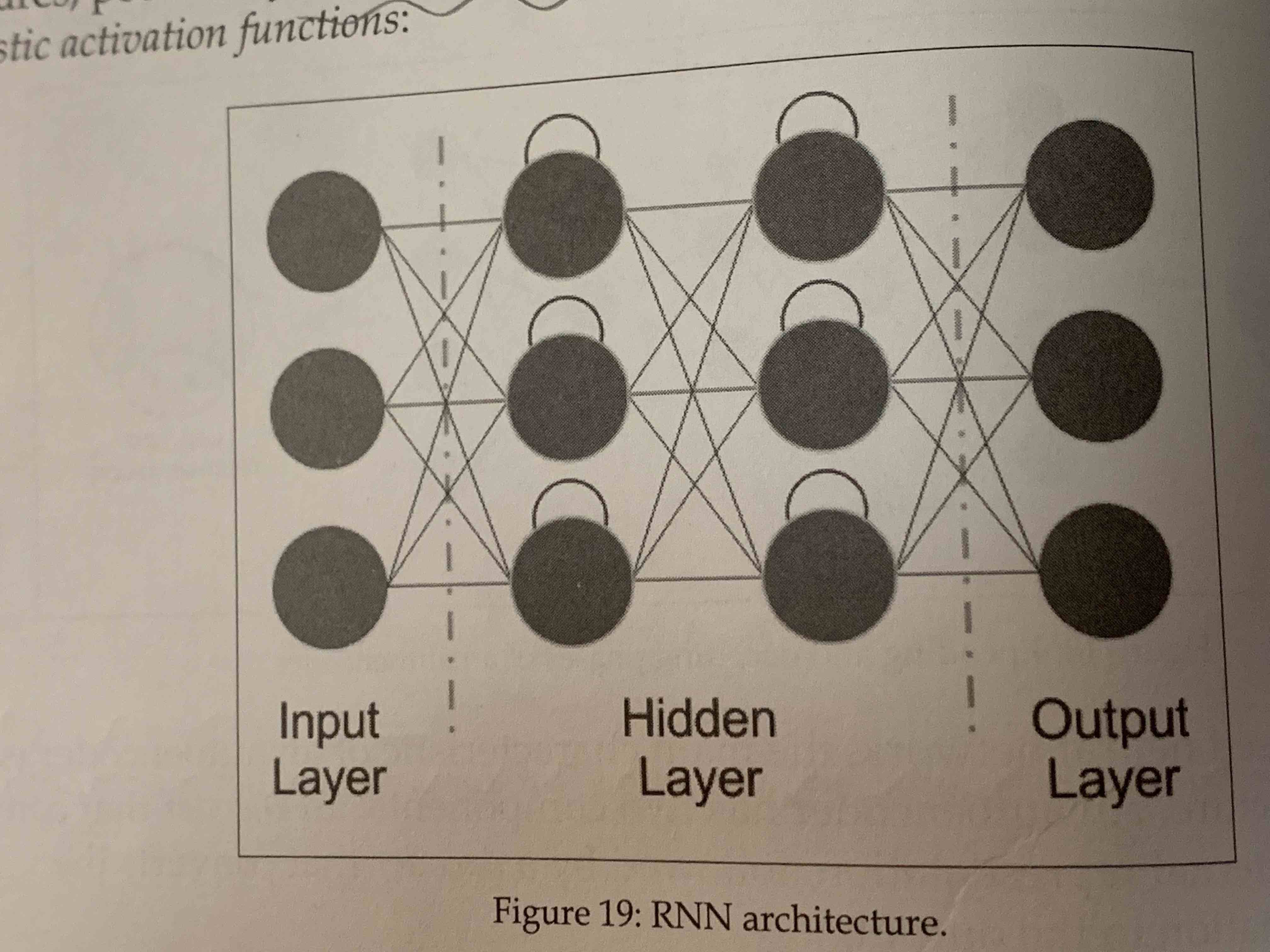
Neural networks can be analogous to the computation of graphs, briefly sorting out the more commonly used neural network architectures:

1. DNN (deep neural networks)

2. CNN (Convolutional neural network)

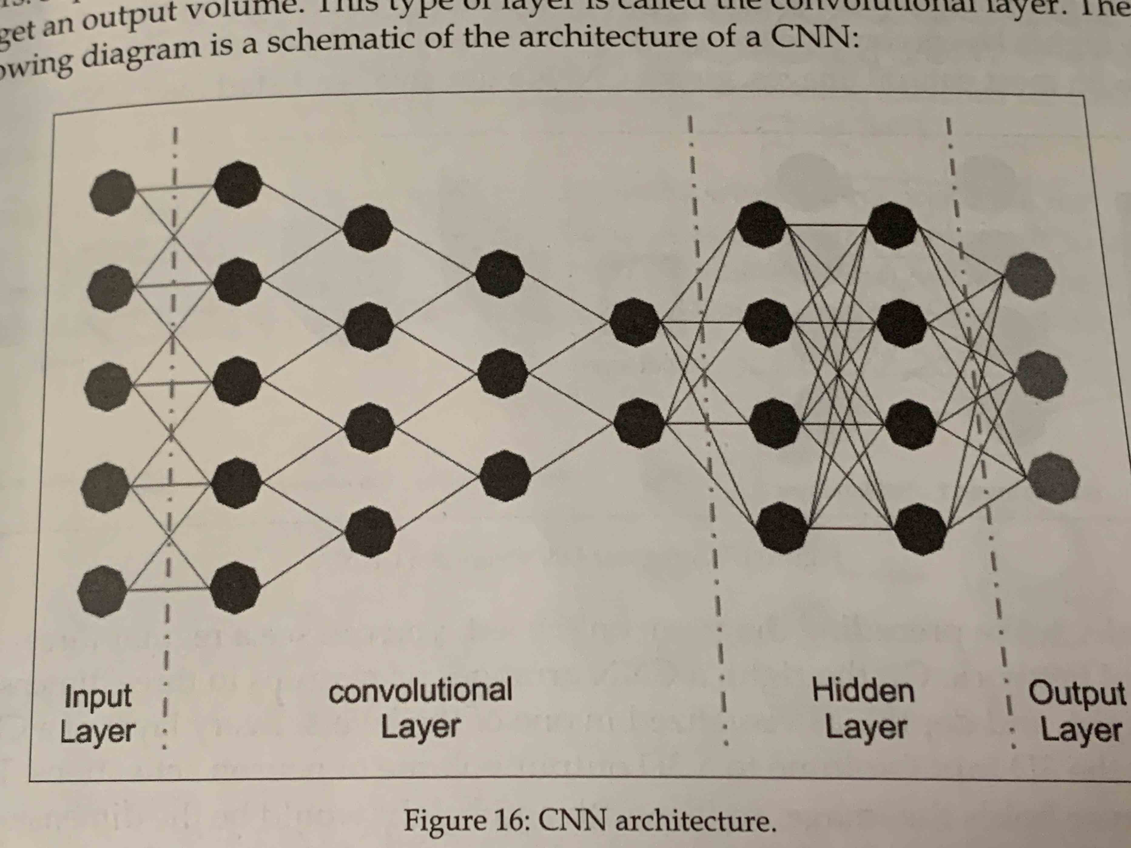
3. RNN (Recurrent neural network)

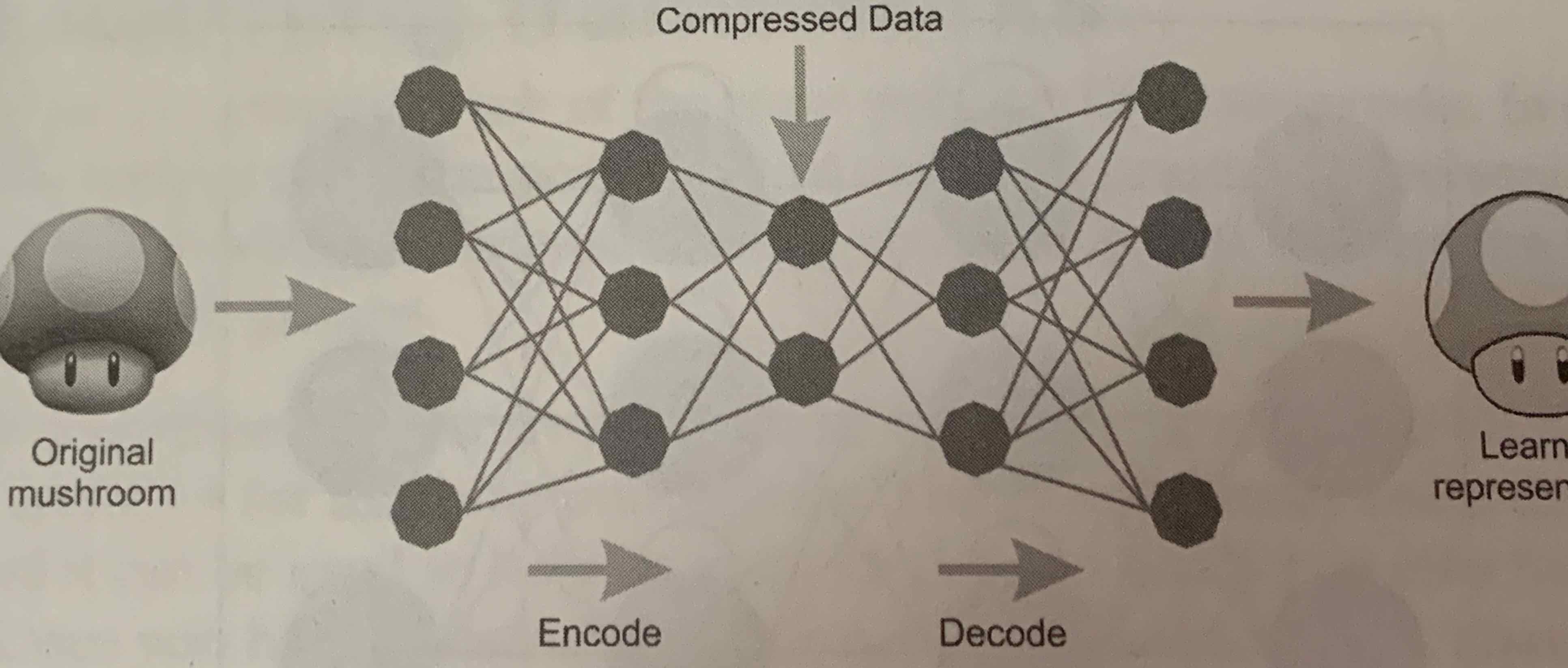
4. AutoEncoders

5. Deep Belief Networks DBNs

6. Restricted Boltzmann Machines (RBMs)

7. Emergent Architectures (EAs)

   • Deep Spatio Temporal Neural Network
   • Mutli-Dimensional Recurrent Neural Network
   • Convolutional AutoEncoders

Artificial Neural Network Algorithms

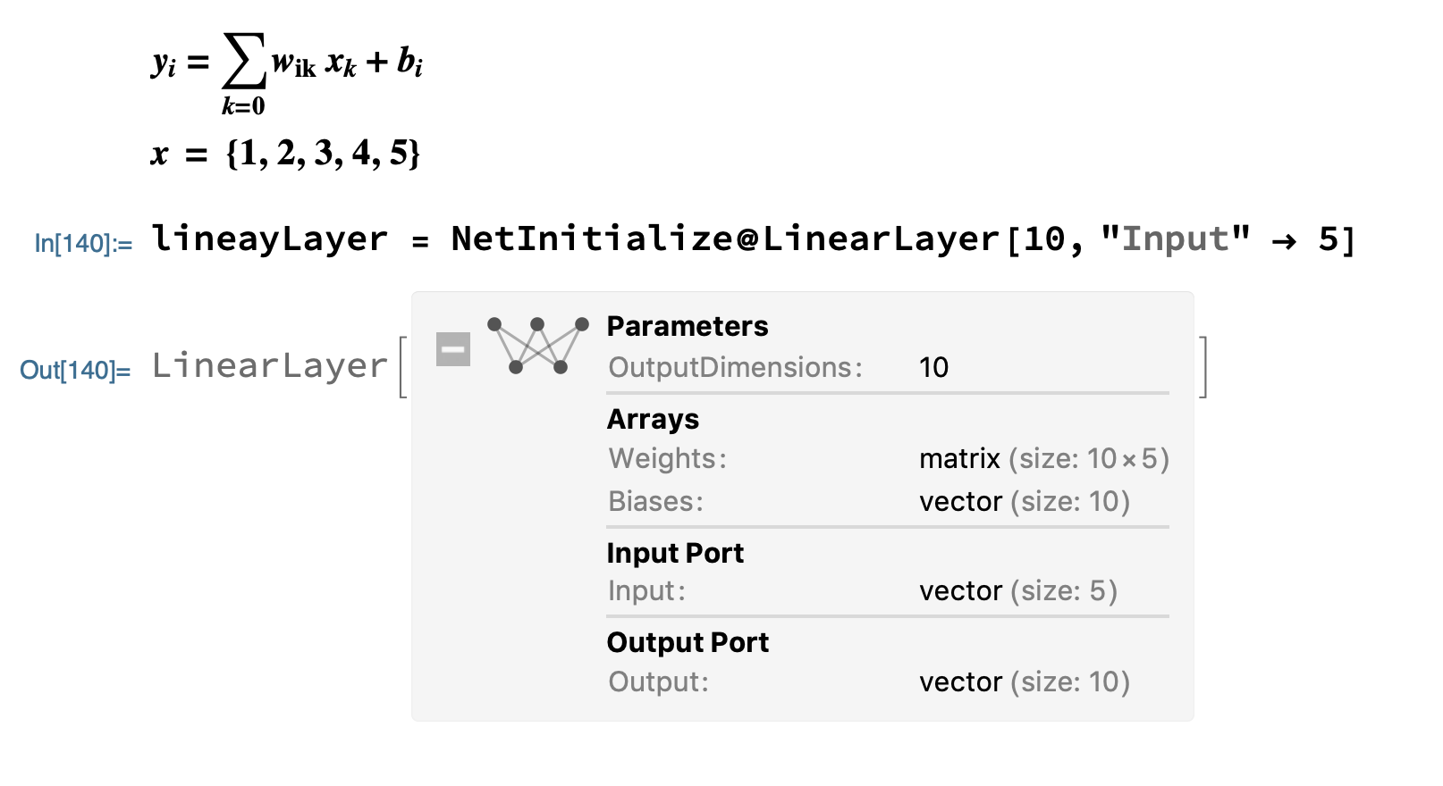
The artificial neural network is computed as above y is the output neuron, x is the input neuron, b is the bias, and w is the connection weight between neurons.

Above we have defined a single layer neural network with output size 10 vector, input vector size 5, weights 10*5 matrix and weight layer size 10.

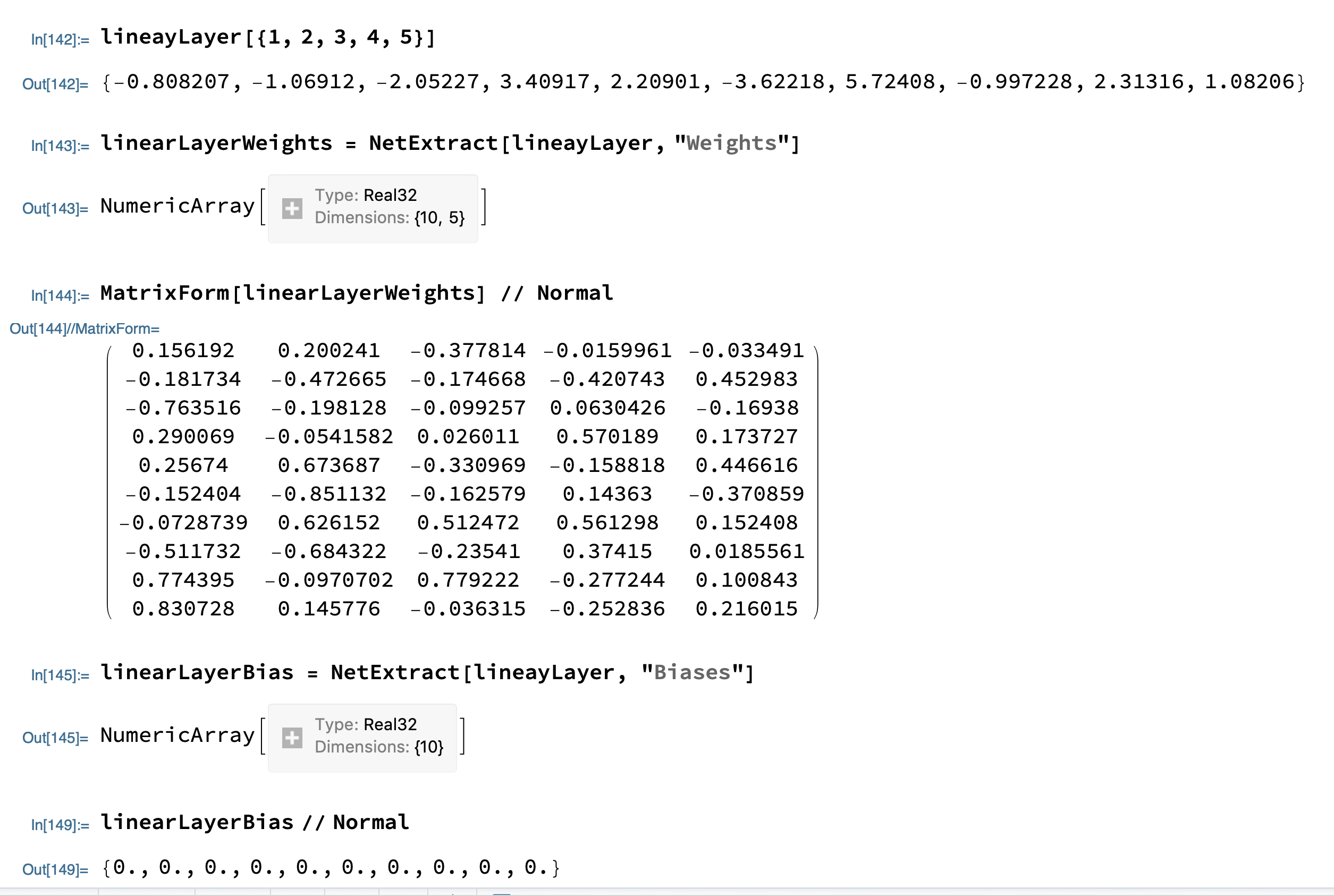
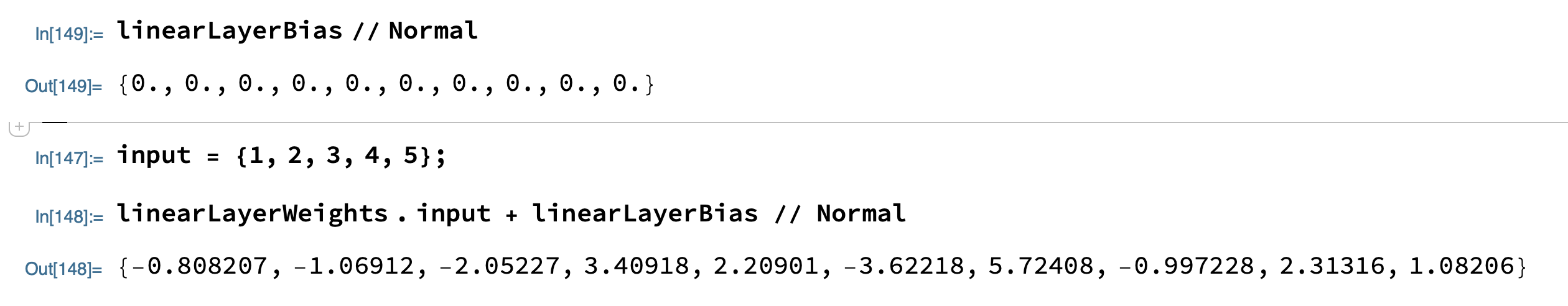
In the above calculation, we input vectors {1,2,3,4,5} into the neural network to get the output as {-0.808207, -1.06912, -2.05227, 3.40917, 2.20901, -3.62218, 5.72408, -0.997228, 2.31316, 1.08206}

From the neural network we obtain the values of the weights and biases, and we can verify that the artificial neural network is calculated as wx + b = y, and the output values obtained from the linearLayerWeights point multiplication input + linearLayerBias are consistent with the above figure.

Gradient descent algorithm

About the gradient calculation:

1. R->R
2. R^(n) -> R^(n)

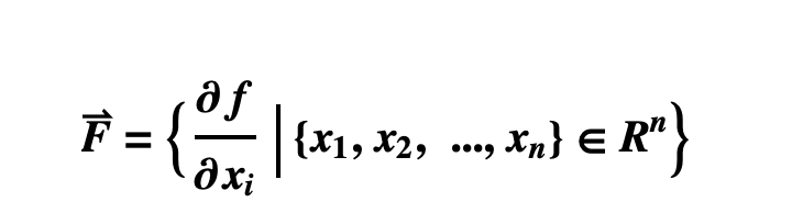
Vector Field:

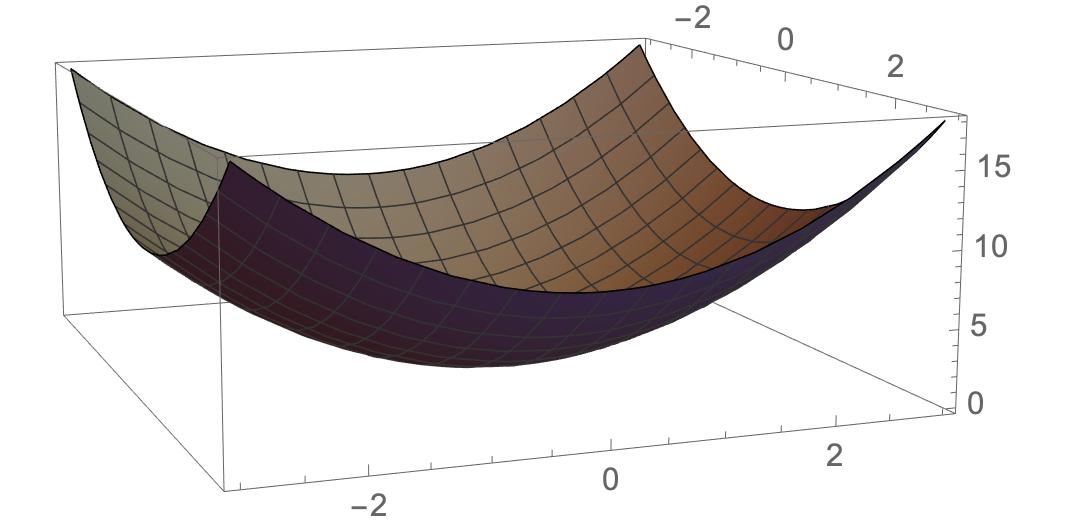
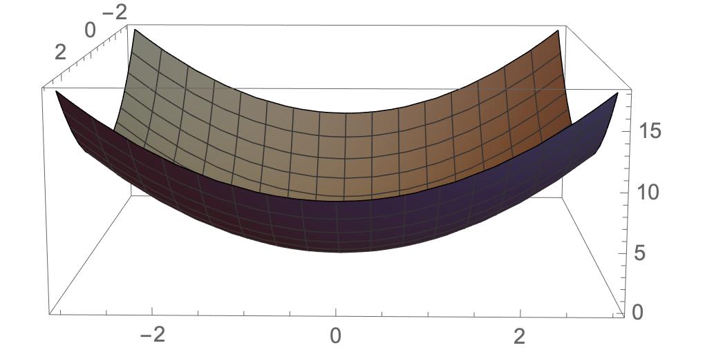
Let z = f(x,y) = x^2 + y^2

Mathematica code is as follows:

f[x_, y_] = x^2 + y^2;
Plot3D[f[x, y], {x, -3, 3}, {y, -3, 3}, PlotStyle -> Gray]

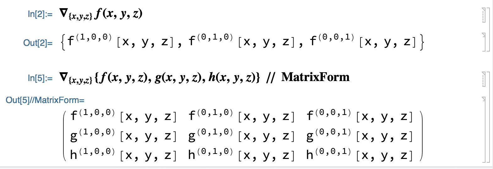
Compute the f(x,y) gradient:

grad = Grad[f[x, y], {x, y}] (* output: {2x, 2y}
VectorDensityPlot[grad, {x, -3, 3}, {y, -3, 3},
 PlotLegends -> Automatic, ColorFunction -> "Rainbow"]

The vector field of gradients can be understood as

The vector field of the gradient of our defined function is shown below, with the colors representing the length of the vectors:

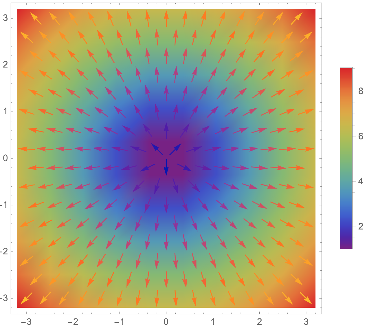
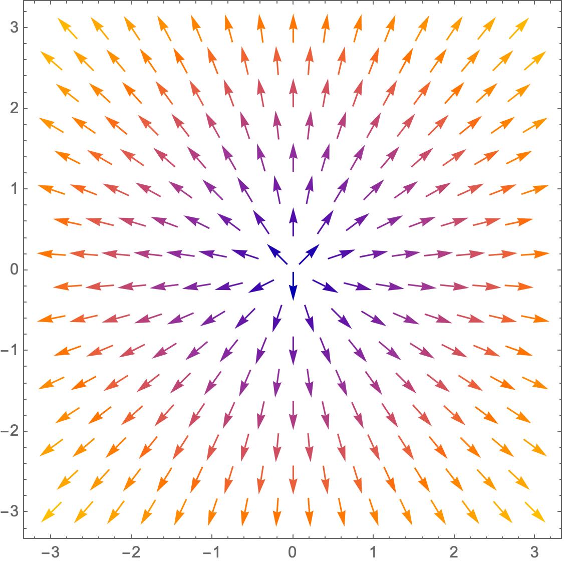
From the graph we can see how the gradient of the function f(x,y) changes at each point as x,y changes.

Find the minimum value based on the gradient :

(* Calculate the gradient *)
grad = Grad[f[x, y], {x, y}]
(* {2 x, 2 y} *)

(* Solve the gradient equation, when the gradient is 0, the function exists as a maximal or minimal value *)
sol = NSolve[grad == {0, 0}, {x, y}, Reals]
(* {{x -> 0, y -> 0}} *)

(* then find the first order derivative of the gradient, which is greater than 0, the function has a minimal value, and less than 0, the function has a maximal value *)
dGrad = Grad[grad, {x, y}]
(* {{2, 0}, {0, 2}} *)

Show[
 Plot3D[f[x, y], {x, -3, 3}, {y, -3, 3},
  PlotStyle -> Opacity[.4]],
 Graphics3D[{PointSize[.04], Red, Point[{x, y, f[x, y]}] /. sol}]]

Get the minimal points of the function {x->0,y->0,z->0}

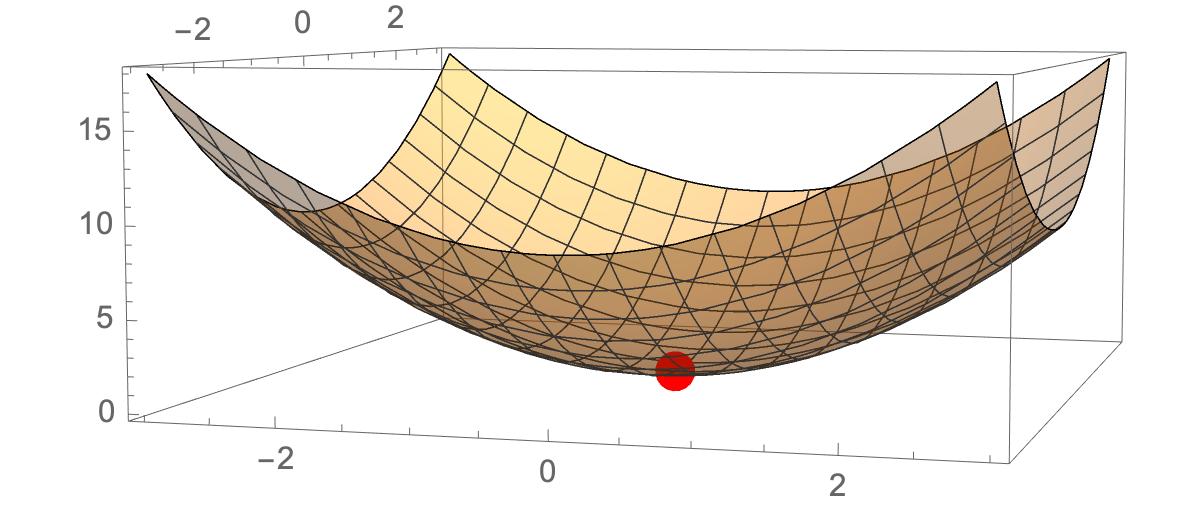
Calculating the gradient of the function and the first order derivative of the gradient will help us determine the extreme point of the function. In neural networks relying on gradient descent algorithms, the values of the weights are changed continuously and iteratively, so that the loss function reaches its extreme value.

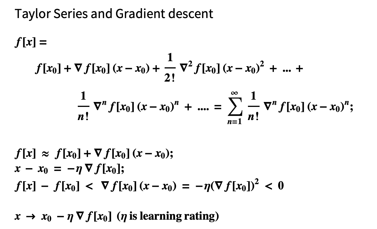
Using the Taylor expansion, we can show that when the variable x is computed according to a decreasing gradient, so that f(x) gradually approaches the extreme value.

Why use an activation function

Why use the activation function, first look at the XOR iso-or operation

{1,1} -> 0
{0,0} -> 0
{1,0} -> 1
{0,1} -> 1

We need to train a model so that the model can predict the computation of XOR.

First model: single model without hidden layers:

data = {{1, 1} -> 0, {0, 0} -> 0, {1, 0} -> 1, {0, 1} -> 1}
net = NetChain[{LinearLayer[1]}]
trained = NetTrain[net, data]
trained[#] & /@ Keys[data]

(* Output: {0.5, 0.5, 0.5, 0.5} *)

We can see that the model is unable to predict simple XOR rules.

The second model adds a hidden layer

net = NetChain[{LinearLayer[16], 1}]

(* Output {0.500014, 0.500002, 0.500009, 0.500006} *)

We still find that the changed model cannot predict the XOR.

The third one continues to increase the number of layers of the hidden layer of the model

net = NetChain[{LinearLayer[16], LinearLayer[16], 1}]

output -> {0.499969, 0.499997, 0.499982, 0.499984}

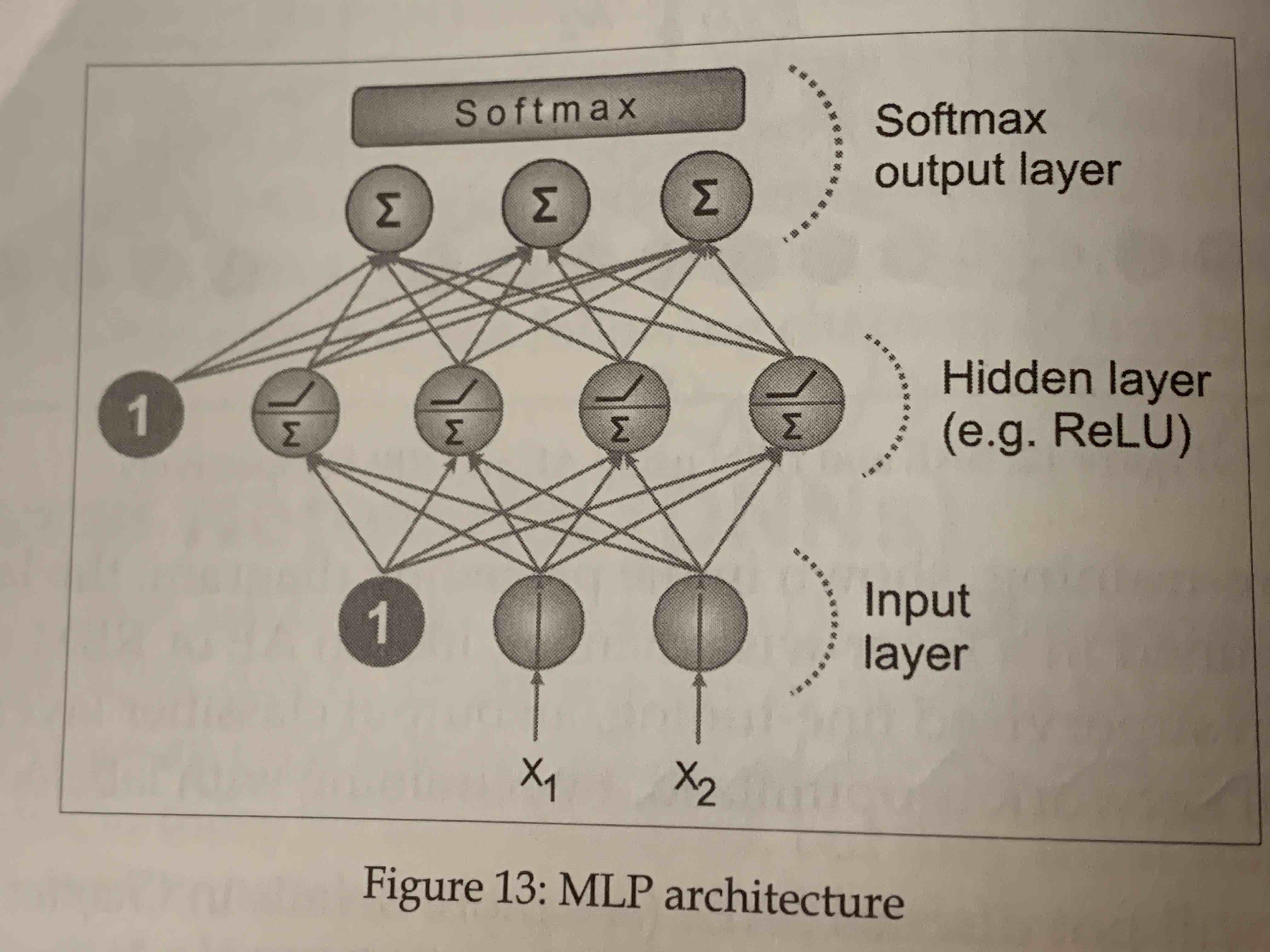
Obviously the model also fails to meet the requirements. Since the algorithm used in the model is a linear regression algorithm with y=wx+b, which cannot represent the XOR operation, it is necessary to add nonlinear characteristics to the network, such as adding the ReLU activation function (rectified linear unit) to the hidden

net = NetChain[{LinearLayer[16], Ramp, 1}]

output -> {4.38886*10^-8, 2.32831*10^-10, 1., 1.}

After adding the nonlinear property, our network can correctly express the XOR operation.

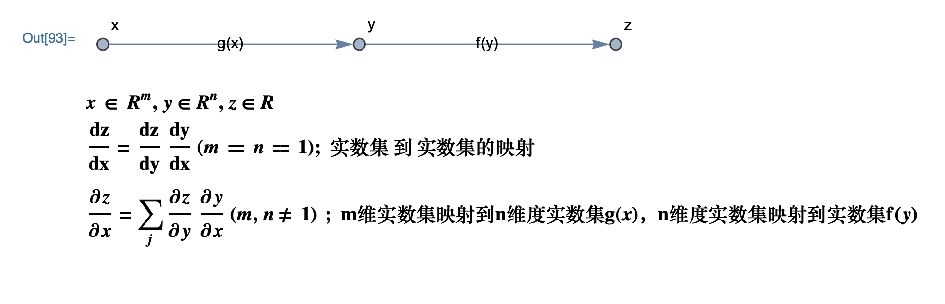
Back-propagation mathematical corollary

First, we introduce the chain derivation rule in calculus as follows:

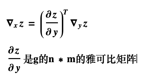
Vector notation:

Activation function

1. Sigmoid

2. Relu

3. tanh

4. softmax

5. cross entropy

Derivation of backpropagation

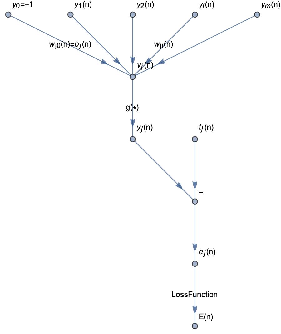
Neural networks are actually computations of graphs in the computation process, first consider artificial neural networks without hidden layers:

According to the theory of supervised learning, we need to calculate the gap between the computed value and the target value, so that the gap is as small as possible. The only parameters that we can adjust in the network are the weights and the threshold value, and in order to minimize the error, we must finely adjust the weights to make the error smaller and smaller.

The backpropagation derivation process is as follows:

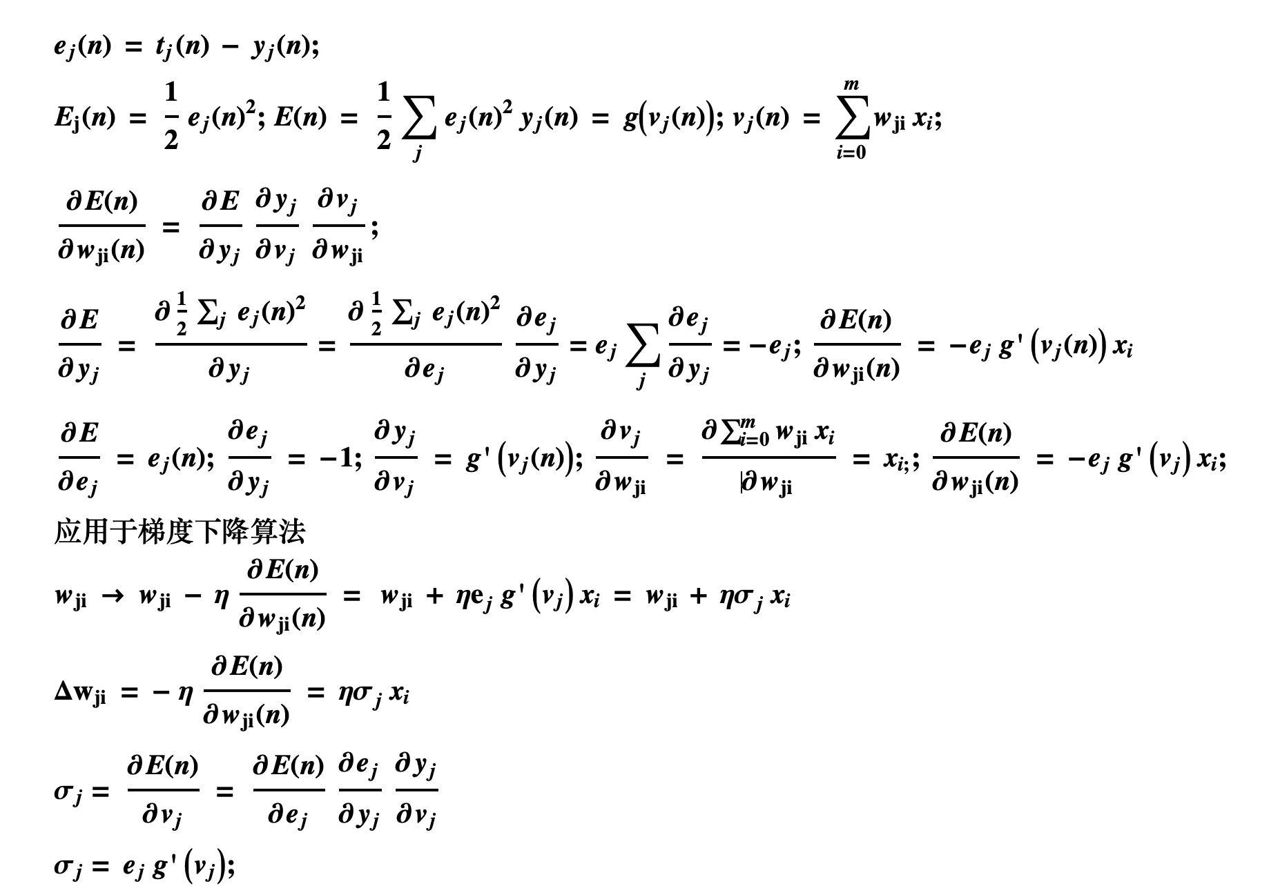
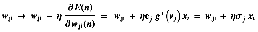
The final adjustment of the weights is calculated as follows:

If xj is the hidden layer in the neural network, as shown below:

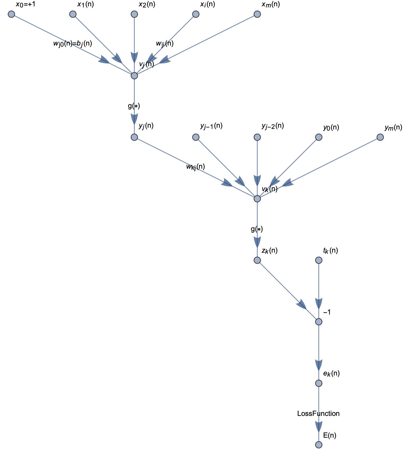
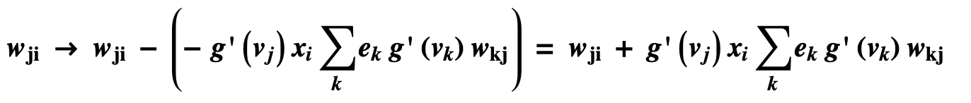
then the derivation of the backpropagation process is shown below:

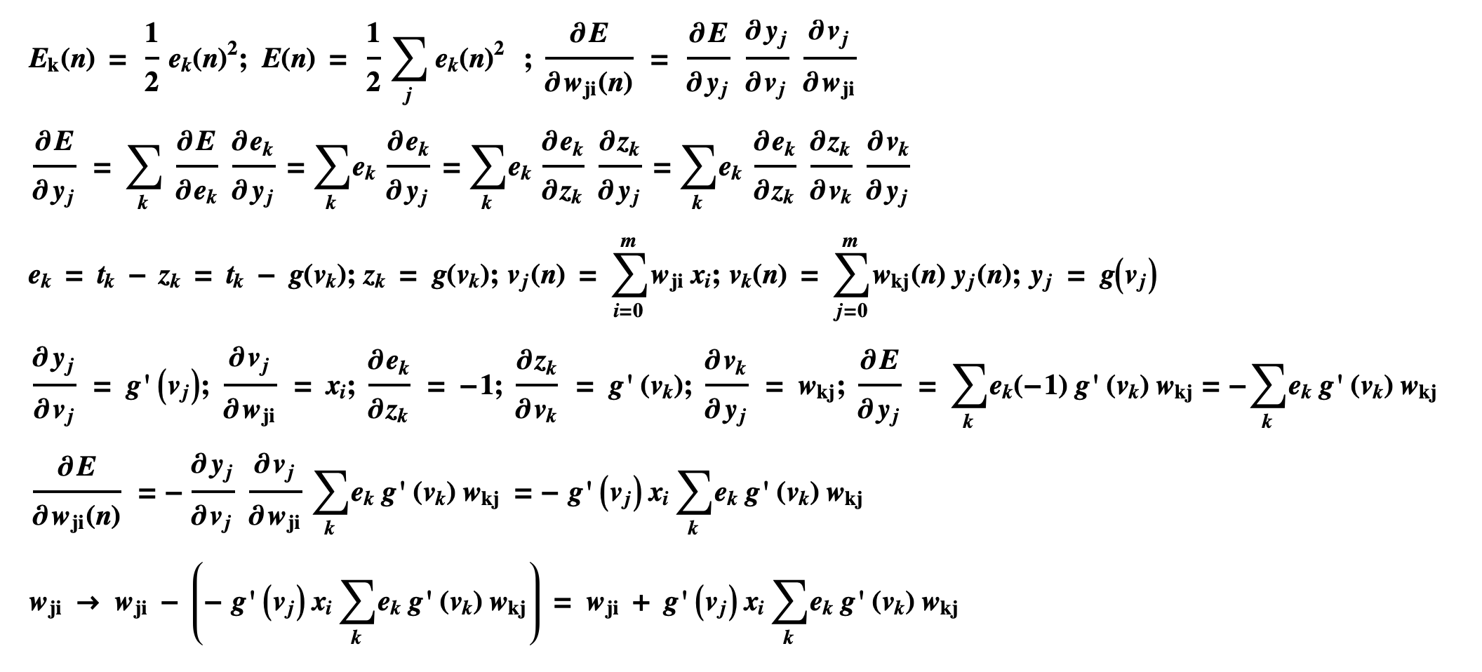
Finally, we adjust the weights of the j-layer network as follows:

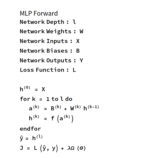
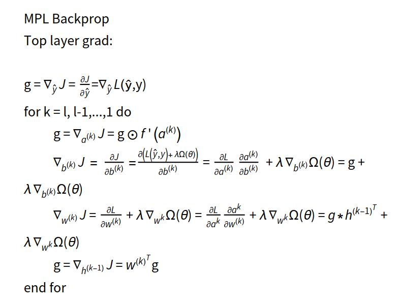
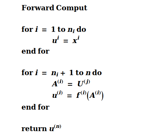
Backpropagation pseudocode

Single-layer neural network computation:

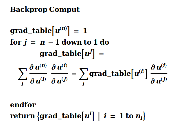
Multi-layer perceptron backwards computation:

Loss function