The animation program code is as follows:
lung-3D.nb
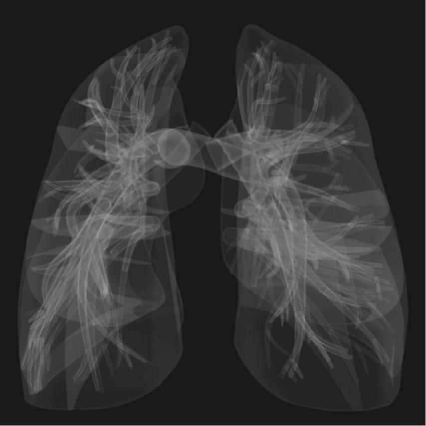
lung3d = AnatomyPlot3D[lung anatomical structure,
PlotTheme->"XRay"]
gif = {};
Do[
image = ImageResize[
Show[lung3d,
ViewPoint -> {3 Cos[x], 3 Sin[x], 0},
ViewAngle -> 20 Degree],
{256, 256}];
gif = Append[gif, image], {x, 0, 2 Pi, 0.1}]
Export["lung-3D.gif", gif, "AnimationRepetitions" -> Infinity ]
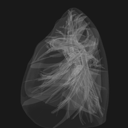
image = ImageResize[
Show[lung3d,
ViewPoint -> {3 Cos[Pi/2], 3 Sin[Pi/2], 0},
ViewAngle -> 20 Degree],
{512, 512}]
Training datasets
Model Architecture
In this paper we will build deep networks that can be trained and deployed on Raspberry pi 4 based on two model frameworks COVID-Net and VGG as references.
Reference Materials
Models
Common Image Model Architectures:
-
MobileNet
-
DenseNet
-
Xception
-
ResNet
-
InceptionV3
-
InceptionResNetV2
-
VGGNet
-
NASNet
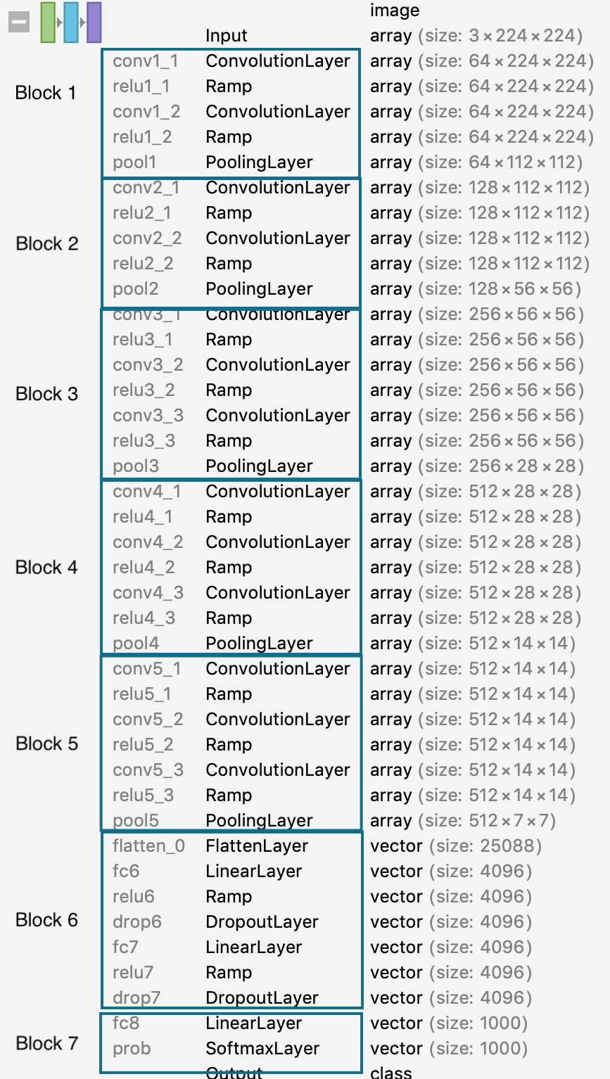
VGG16
Model Architecture
COVID-NET
Model Architecture
Prototype Testing
VGG16 迁移学习
The dataset used is covid19-radiography-database.
The NoteBook link is as follows:
Mathematica VGG16 Transfer Learning Code
After training the model, we used the test set to measure the model’s accuracy at 94%.
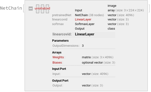
Here we use a migration learning approach to accelerate the training of the model by removing the top layer of the pre-trained VGG16 model and adding three classified linear layers, {“COVID-19”, “NORMAL”, “VIRAL”}, and training only the parameters of the linearcovid layer.
ConfusionMatrixPlot of the final model:
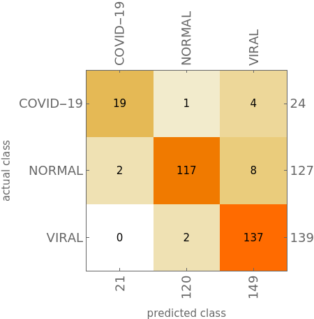
In this prototype test, we used VGG16 to classify the X-ray images into three subsets, namely {“COVID-19”, “NORMAL”, “VIRAL”}, the total number of images in the dataset is 2905, and Normal means normal. The lung pictures, VIRAL refers to other pictures of viral infections of pneumonia disease. There are only 219 of these Covid-19 images, and the training set, validation set, and test set occupancy is divided 8:1:1.
Finally, an X-Ray image of a Covid-19 patient’s lung was obtained randomly from the Internet and validated in the model:
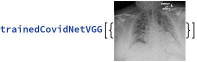
The resulting result is COVID-19.
The above test results are only a vague notion, since our data set is only 2k.
Enhanced VGG16
What we need to explore next is how to manually generate the entire VGG16 deep learning architecture, copy the pre-trained weights into the VGG16 network we created, and then adopt a hierarchical training method to train one feature layer and freeze the other layers. This is done in mathematica.
- Create VGG16 Model
vgg16Layers = Association[{
    (* Block 1 *)
    1 -> {
      "features" -> 64,
      "kernel" -> {3, 3},
      "padding" -> 1,
      "pooling" -> {
        "kernel" -> {2, 2},
        "stride" -> {2, 2}},
      "layers" -> {"Conv1" ->
         "Ramp1" -> "Conv2" -> "Ramp2" -> "Pooling"} },

    (* Block 2 *)
    2 -> {
      "features" ->  128,
      "kernel" -> {3, 3},
      "padding" -> 1,
      "pooling" -> {
        "kernel" -> {2, 2},
        "stride" -> {2, 2}},
      "layers" -> {"Conv1" ->
         "Ramp1" -> "Conv2" -> "Ramp2" -> "Pooling"}},
    (* Block 3 *)
    3 -> {
      "features" -> 256,
      "kernel" -> {3, 3},
      "padding" -> 1,
      "pooling" -> {
        "kernel" -> {2, 2},
        "stride" -> {2, 2}},
      "layers" -> {"Conv1" ->
         "Ramp1" ->
          "Conv2" -> "Ramp2" -> "Conv3" -> "Ramp3" ->  "Pooling"}},
    (* Block 4 *)
    4 -> {
      "features" -> 512,
      "kernel" -> {3, 3},
      "padding" -> 1,
      "pooling" -> {
        "kernel" -> {2, 2},
        "stride" -> {2, 2}},
      "layers" -> {"Conv1" ->
         "Ramp1" ->
          "Conv2" -> "Ramp2" -> "Conv3" -> "Ramp3" ->  "Pooling"}},
    (* Block 5 *)
    5 -> {
      "features" -> 512,
      "kernel" -> {3, 3},
      "padding" -> 1,
      "pooling" -> {
        "kernel" -> {2, 2},
        "stride" -> {2, 2}},
      "layers" ->
       {"Conv1" ->
         "Ramp1" ->
          "Conv2" -> "Ramp2" -> "Conv3" -> "Ramp3" ->  "Pooling"}}
    }];
The entire VGG16 is focused on the convolutional layer, which is structured as shown in the above code:
feature layer n -> {“features” -> number of output features, “kernel” -> convolutional kernel size, “padding” -> padding size, “pooling” -> {“kernel” -> pooling layer kernel, “stride” -> pooling layer > step size, “layers” -> the feature layer connection structure}}
The convolution layer has 5 modules in total, the kernel of each convolution layer is {3,3}, the move step is {1,1}, the padding is {{1,1},{1,1}}, the padding can be interpreted as the offset between the start and end positions, for example, if we enter > a two-dimensional image, we can understand the padding as {{x_begin, x_end}, {{y_begin, y_end}}.
Generating the VGG16 model:
(* This function parses our VGG16 model tree above in a tail recursive manner and generates a list of hierarchies. *)
reMapLayers[layers_, return_, blockInfo_] := Module[{key, values, res},
  If[MatchQ[layers, KeyValuePattern[_ -> _]],
   key = Keys[layers][[1]];
   values = Values[layers];
   If[StringContainsQ[key, "conv", IgnoreCase -> True],
    res =
     Append[return, key -> ConvolutionLayer @@ blockInfo["conv2"]],
    If[StringContainsQ[key, "ramp", IgnoreCase -> True],
     res = Append[return, key -> ElementwiseLayer["ReLU"]],
     If[StringContainsQ[key, "pool", IgnoreCase -> True],
      res = Append[return, key -> PoolingLayer @@ blockInfo["pooling"]]
      ]]],
   If[StringContainsQ[layers[[1]], "pool", IgnoreCase -> True],
    res =
     Append[return,
      layers[[1]] -> PoolingLayer @@ blockInfo["pooling"]];
    Return[res]]];
  reMapLayers[values, res, blockInfo]]
(* This function generates the model layer for each Block by calling reMapLayers. *)

vgg16Unit[nBlock_] := Module[{conv2, pooling, blockinfo, layers},
  conv2 = {"features", "kernel", PaddingSize -> "padding"} /.
    vgg16Layers[nBlock];
  pooling = {"kernel", "stride"} /. (
     "pooling" /. vgg16Layers[nBlock] );
  blockinfo = <|"conv2" -> conv2, "pooling" -> pooling|>;
  layers = "layers" /. vgg16Layers[nBlock];
   NetChain[reMapLayers[layers, {}, blockinfo]]
  ]
(* Combined with the functions provided above, createVGG16Model is used to generate the final VGG16 model, called as:

vgg16net =
 createVGG16Model[input -> {224, 224, 3}, output -> {"cat", "dog"},
  transferLearning -> True]

input: the dimension of the input image, (H * W * Channels)
output: The corresponding label of the data.
transferLearning -> True: Indicates that the model uses transfer learning techniques, and the weights of the newly generated model will be multiplexed with the weights of the already trained VGG16 model.

*)

Options[createVGG16Model] = {input -> {224, 224, 3},
   output -> {"cat", "dog"}, transferLearning -> False};
createVGG16Model[OptionsPattern[]] :=
 Module[{blocks, topLayers, net, lossnet, trainedNet, dims, channels,
   extractConvInfo, preModel, nchannels, conv1weights, conv1biases,
   combinRGBToGray,
   input = OptionValue[input],
   output = OptionValue[output],
   transferLearning = OptionValue[transferLearning]},
  (* preTrained Model Import *)

  preModel :=
   NetModel["VGG-16 Trained on ImageNet Competition Data"];

  (* conver RGB Channel conv1 to Grayscale conv1 *)

  combinRGBToGray[rgbC_] := Module[{r, g, b, gray},
    r = rgbC[[1]];
    g = rgbC[[2]];
    b = rgbC[[3]];
    gray =  0.2989 r + 0.5870 g + 0.1140 b;
    {gray}];

  (* extract preTrained Model Weights and Biases *)

  extractConvInfo[preTrainedmodel_] :=
   Module[{data = {}, keys, allInfo},
    allInfo = NetExtract[preTrainedmodel, All];
    keys =
     Select[Keys[allInfo],
      StringContainsQ[#, "conv", IgnoreCase -> True] &];
     # ->  allInfo[#]  &  /@ keys];

  (* Set dims and channels, input and output *)

  dims = input[[1 ;; 2]];
  nchannels = input[[3]];
  channels = If[nchannels == 3, "RGB", "Grayscale"];
  trainedNet =
   If[transferLearning, Association[extractConvInfo[preModel]],
    None];
  input = NetEncoder[{"Image", dims, ColorSpace -> channels}];
  output = NetDecoder[{"Class", output}];
  (* top layers *)
  topLayers = NetChain[{
     "fc0" -> FlattenLayer[],
     "fc1" -> LinearLayer[4096],
     "ramp1" -> Ramp,
     "drop1" -> DropoutLayer[],
     "fc2" -> LinearLayer[4096],
     "ramp2" -> Ramp,
     "drop2" -> DropoutLayer[],
     "fc4" -> LinearLayer[],
     "soft" -> SoftmaxLayer[]
     }];
  (* VGG16 Blocks *)

  blocks = <|
    "arg" -> ImageAugmentationLayer[dims],
    "block1" -> vgg16Unit[1],
    "block2" -> vgg16Unit[2],
    "block3" -> vgg16Unit[3],
    "block4" -> vgg16Unit[4],
    "block5" -> vgg16Unit[5],
    "top" -> topLayers
    |>;
  net  = NetGraph[
    blocks,
    {"arg" ->
      "block1" ->
       "block2" -> "block3" -> "block4" -> "block5" -> "top"},
    "Input" -> input,
    "Output" -> output];
  If[transferLearning,
   If[Join[dims, {nchannels}] == {224, 224, 3},
    net =
     NetReplacePart[net, {"block1", "Conv1"} -> trainedNet["conv1_1"]],
    If[Join[dims, {nchannels}] == {224, 224, 1},
     conv1weights = NetExtract[trainedNet["conv1_1"], "Weights"];
     conv1biases = NetExtract[trainedNet["conv1_1"], "Biases"];
     conv1weights =
      NumericArray@Map[combinRGBToGray, Normal[conv1weights]];
     net =
      NetReplacePart[
       net, {"block1", "Conv1", "Weights"} -> conv1weights];
     net =
      NetReplacePart[
       net, {"block1", "Conv1", "Biases"} -> conv1biases]]];
   net = NetReplacePart[
     net, {"block1", "Conv2"} -> trainedNet["conv1_2"]];
   net = NetReplacePart[
     net, {"block2", "Conv1"} -> trainedNet["conv2_1"]];
   net = NetReplacePart[
     net, {"block2", "Conv2"} -> trainedNet["conv2_2"]];
   net = NetReplacePart[
     net, {"block3", "Conv1"} -> trainedNet["conv3_1"]];
   net = NetReplacePart[
     net, {"block3", "Conv2"} -> trainedNet["conv3_2"]];
   net = NetReplacePart[
     net, {"block3", "Conv3"} -> trainedNet["conv3_3"]];
   net = NetReplacePart[
     net, {"block4", "Conv1"} -> trainedNet["conv4_1"]];
   net = NetReplacePart[
     net, {"block4", "Conv2"} -> trainedNet["conv4_2"]];
   net = NetReplacePart[
     net, {"block4", "Conv3"} -> trainedNet["conv4_3"]];
   net = NetReplacePart[
     net, {"block5", "Conv1"} -> trainedNet["conv5_1"]];
   net = NetReplacePart[
     net, {"block5", "Conv2"} -> trainedNet["conv5_2"]];
   net = NetReplacePart[
     net, {"block5", "Conv3"} -> trainedNet["conv5_3"]];
   net,
   net]]
Finally, we try to migrate and learn catVSdog using the newly generated model to test whether our model works properly.
Options[createVGG16Model]

{input -> {224, 224, 3}, output -> {"cat", "dog"},
 transferLearning -> False}

vgg16net =
 createVGG16Model[input -> {224, 224, 3}, output -> {"cat", "dog"},
  transferLearning -> True]
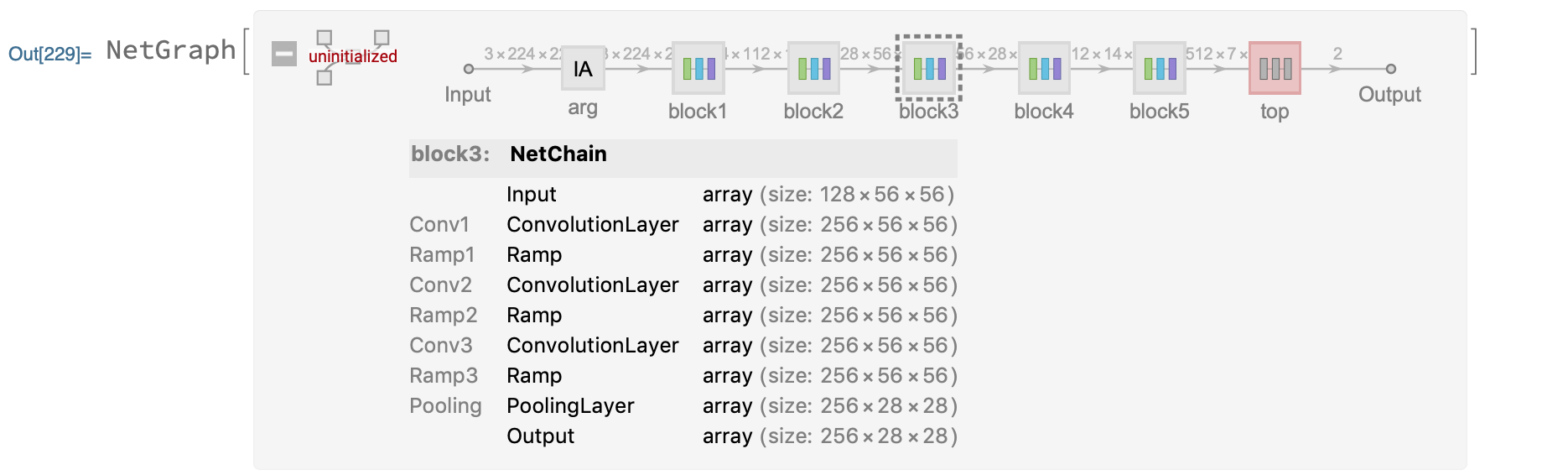
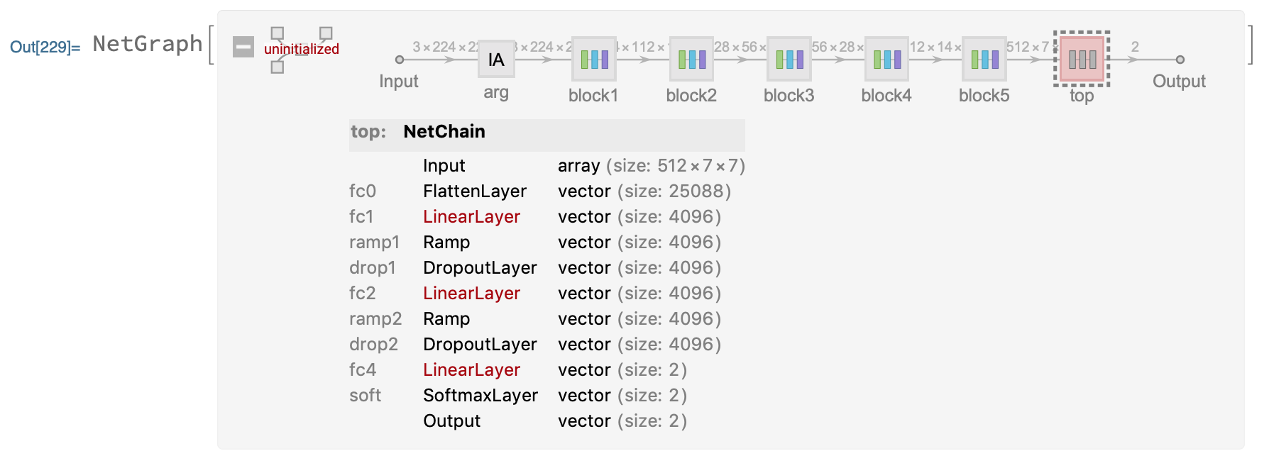
The structure of the model is shown in the figure above, divided into 6 modules, {block1,block2,block3,block4,block5,top}, where the weights and deviations of block{1~5} convolutional layer have been set, and the weights and deviations of top layer> have not been initialized.
Let’s test the accuracy of the model by training only one round:
LearningRateMultipliers -> {“block” -> 0} weights used to freeze the block layer.
trainedVgg16 =
 NetTrain[vgg16net, traingDataFilesSplit, All,
  ValidationSet -> validDataFilesSplit,
  TrainingProgressReporting -> "Panel", BatchSize -> 32,
  LearningRateMultipliers -> {"block1" -> 0, "block2" -> 0,
    "block3" -> 0, "block4" -> 0, "block5" -> 0, _ -> 1},
  MaxTrainingRounds -> 1
  ]
The training results are as follows:
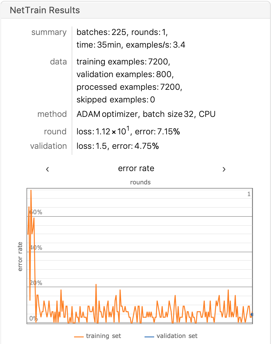
Use a test set to observe the accuracy of the model:
NetMeasurements[trainedVgg16["TrainedNet"], testDataFiles, "Accuracy"]

0.954

There are 84 sheets of cat that are actually mistaken for dog.
Verify that the freeze layer is indeed frozen during the training process:

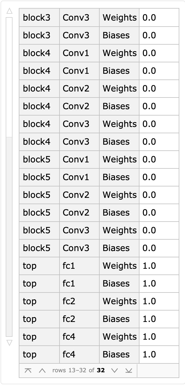
It can be determined that the learning rate is 0 for all Block layers and only 1 for the top layer.
Is there any improved way to continue to improve the accuracy of the model?
Refer to the paper [Covid-19 detection using CNN transfer learning from X-ray Images](https://www.medrxiv.org/content/10.1101/2020.05. 12.20098954v2.full.pdf)
The following CNN architecture is used in the paper
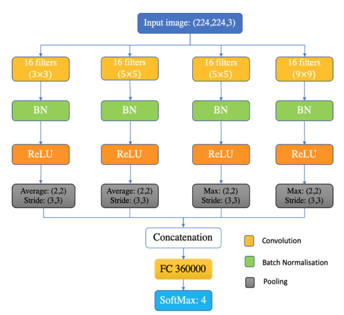
XConvidNet = NetInitialize[NetGraph[<|
    "concat" -> CatenateLayer[],
    "conv1" -> ConvolutionLayer[16, 3, PaddingSize -> 1],
    "bn1" -> BatchNormalizationLayer[],
    "relu1" -> Ramp,
    "pooling1" -> PoolingLayer[{2, 2}, {3, 3}],

    "conv2" -> ConvolutionLayer[16, 5, PaddingSize -> 2],
    "bn2" -> BatchNormalizationLayer[],
    "relu2" -> Ramp,
    "pooling2" -> PoolingLayer[{2, 2}, {3, 3}],

    "conv3" -> ConvolutionLayer[16, 5, PaddingSize -> 2],
    "bn3" -> BatchNormalizationLayer[],
    "relu3" -> Ramp,
    "pooling3" -> PoolingLayer[{2, 2}, {3, 3}],

    "conv4" -> ConvolutionLayer[16, 9, PaddingSize -> 5],
    "bn4" -> BatchNormalizationLayer[],
    "relu4" -> Ramp,
    "pooling4" -> PoolingLayer[{2, 2}, {3, 3}],

    "fc" -> FlattenLayer[],
    "linear0" -> LinearLayer[],
    "Soft" -> SoftmaxLayer[]
    |>, {
    "conv1" -> "bn1" -> "relu1" -> "pooling1" -> "concat",
    "conv2" -> "bn2" -> "relu2" -> "pooling2" -> "concat",
    "conv3" -> "bn3" -> "relu3" -> "pooling3" -> "concat",
    "conv4" -> "bn4" -> "relu4" -> "pooling4" -> "concat",
    "concat" -> "fc" -> "linear0" -> "Soft"},
   "Input" -> NetEncoder[{"Image", {224, 224}, ColorSpace -> "RGB"}],
   "Output" -> NetDecoder[{"Class", {"cat", "dog"}}]]]
This inspires us whether we can combine two or more CNN models in the same way, extend the domain of the features, and connect the final output features of multiple CNN models into the same > tensor by transfer learning, and finally perform the Flatten operation on the tensor, we just need to train “fc”->“linear0” parameters.
Next, we test the above architecture with Resnet-50 and VGG16, generate the Resnet-50 model architecture and copy the pre-trained Resnet50 weights into the model, just like the VGG16 model, where we directly use the pre-trained ResNet50 from Wolfram Neural Network.
newNet = NetGraph[<|

   "arg" ->
    ImageAugmentationLayer[{224, 224},
     "ReflectionProbabilities" -> {0.5, 0.5}],
   "resNet" -> NetTake[resNet, {"conv1", "5c"}] ,
   "vgg" -> NetTake[vgg16net, {"block1", "block5"}],
   "concat" -> CatenateLayer[],
   "pooling" -> PoolingLayer[{7, 7}, "Function" -> Mean],
   "fc0" -> FlattenLayer[],
   "fc1" -> LinearLayer[500],
   "fc2" -> LinearLayer[2],
   "soft" -> SoftmaxLayer[]|>,
  {NetPort["Input"] -> "arg" ->  {"resNet", "vgg"},
   {"resNet", "vgg"} ->
    "concat" -> "pooling" -> "fc0" -> "fc1" -> "fc2" -> "soft"},
  "Input" -> NetEncoder[{"Image", {224, 224}, ColorSpace -> "RGB"}],
  "Output" -> NetDecoder[{"Class", {"cat", "dog"}}]]
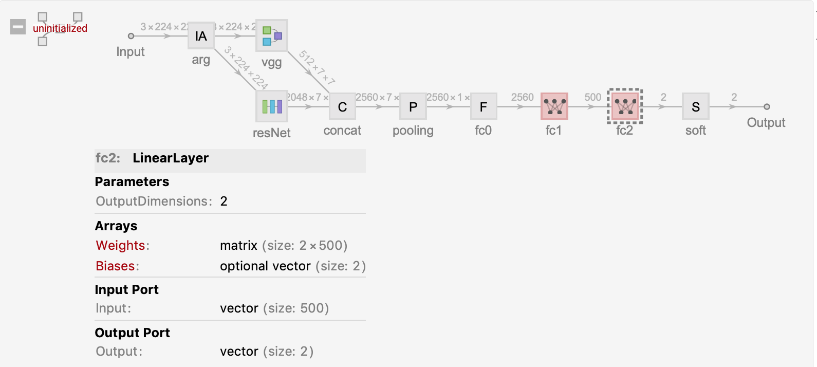
We only need to train the parameters of fc1 fc2 two linear layers, and fix the weights of other layers. We compare our results with the above VGG16 training.
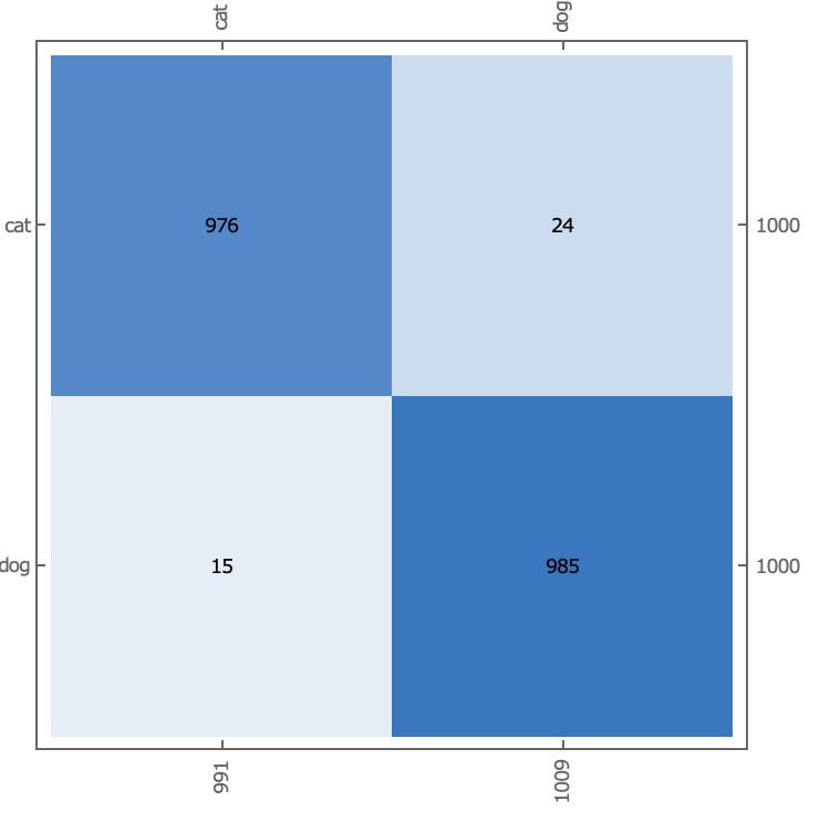
On the entire test set, we calculate the accuracy and confusion matrix of the model, and we can see a significant improvement in the model, with an accuracy of 98.05%.
NetMeasurements[trainedVgg16["TrainedNet"], testDataFiles, "Accuracy"]

0.9805
Currently we are using VGG16, ResNet-50, Mix-VGG16/ResNet-50. The following is the Mathematica code to build ResNet-50, and separately verify that catVSdog has been trained from scratch on ResNet-50 and that we have built it from scratch on ResNet-50. Use migration to learn the effects of both.
Covid-Net
- Reference Papers
- Architecture Design
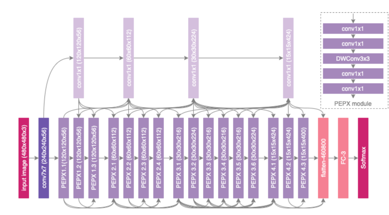
The Covid-Net architecture uses the Lightweight design pattern, which uses the PEPX (projection-expansion-projection-extension) pattern, where each PEPX module contains the following five parts Sub:
-
first stage projection -> 1 * 1 convolutional kernel, mapping input features to low latitudes
-
expansion -> 1 * 1 convolutional kernel, expansion of feature attributes will map features to high dimensionality
Depth-wise representation -> 3*3 convolutional kernels are used to reduce computational complexity while preserving important features.
-
second-stage projection -> lower dimensionality of feature input using 1*1 convolutional kernel
-
extension -> 1*1 convolutional core, extension output to high latitude, as the final output
Model Building:
Based on the above description, let’s build the basic architecture of PEPX.
pepxModel[inChannel_, outChannel_] := Module[
  {model },
  model = NetChain[{
     ConvolutionLayer[Floor[ inChannel/ 2], {1, 1}],
     ConvolutionLayer[IntegerPart[3 * inChannel / 4], {1, 1}],
     ConvolutionLayer[IntegerPart[3 * inChannel / 4], {3, 3},
      PaddingSize -> {1, 1}],
     ConvolutionLayer[Floor[inChannel / 2], {1, 1}],
     ConvolutionLayer[outChannel, {1, 1}]}];
  model]
NetGraph[<|
  "inputConv1" -> NetChain[{
     ConvolutionLayer[56, {7, 7}, "Stride" -> {2, 2},
      PaddingSize -> {3, 3}],
     Ramp,
     PoolingLayer[{3, 3}, PaddingSize -> {1, 1}]}],
  "pepx1.1" -> pepxModel[56, 56],
  "pepx1.2" -> pepxModel[56, 56],
  "pepx1.3" -> pepxModel[56, 56],
  "conv1_1x1" -> ConvolutionLayer[56, {1, 1}, "Stride" -> {2, 2}],
  "conv1_1*1+pepx1.1"  -> TotalLayer[],
  "conv1_1*1+pepx1.{1,2}" -> TotalLayer[]
  |>,
 {
  "inputConv1" ->  "conv1_1x1" -> "pepx1.1" ,
  {"pepx1.1", "conv1_1x1"} -> "conv1_1*1+pepx1.1" -> "pepx1.2",
  {"pepx1.1", "conv1_1x1", "pepx1.2"} ->
   "conv1_1*1+pepx1.{1,2}"  -> "pepx1.3"
  },
 "Input" -> NetEncoder[{"Image", {480, 480}, ColorSpace -> "RGB"}]]
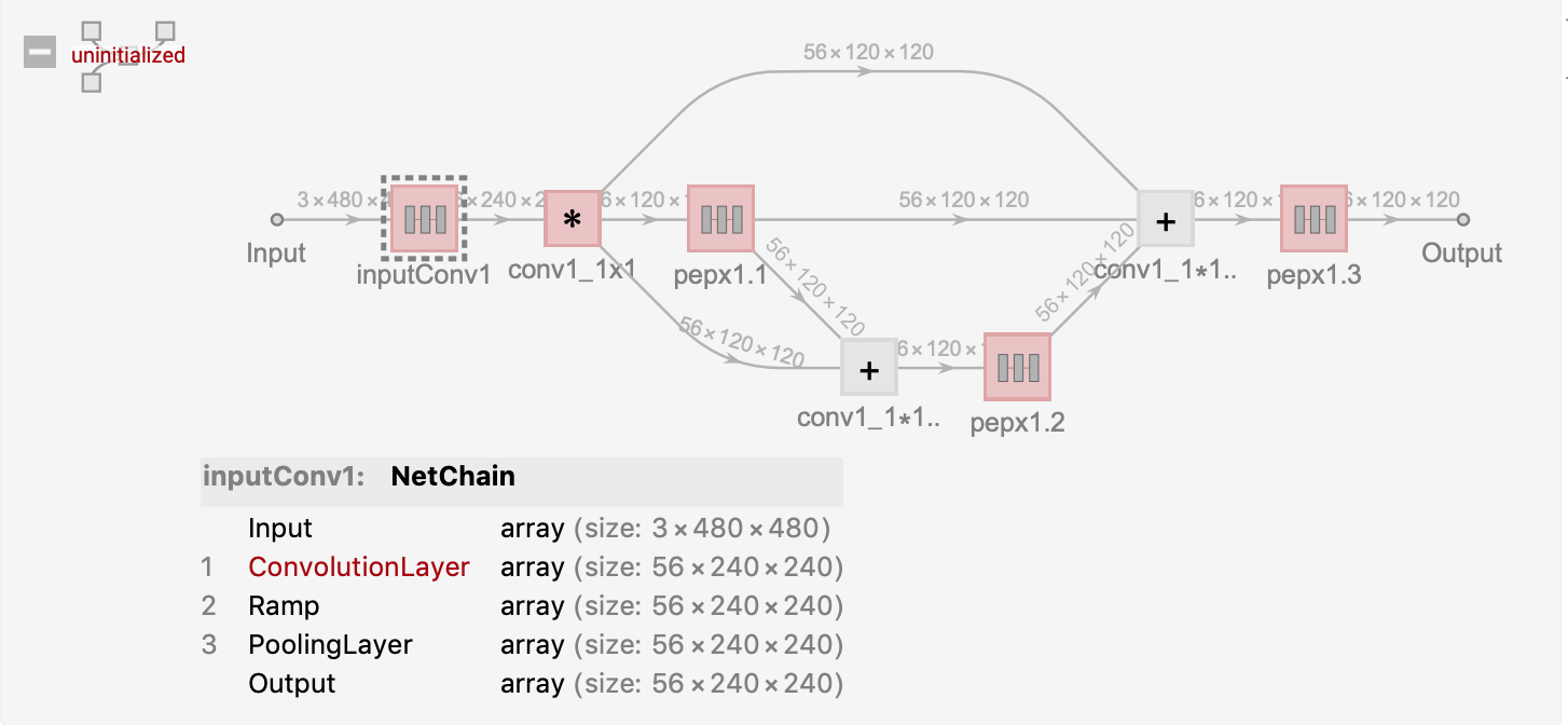
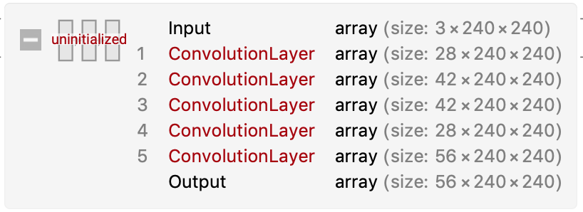
Since Covid-Net’s model building code is not publicly available, we created the test model manually in mathematica.
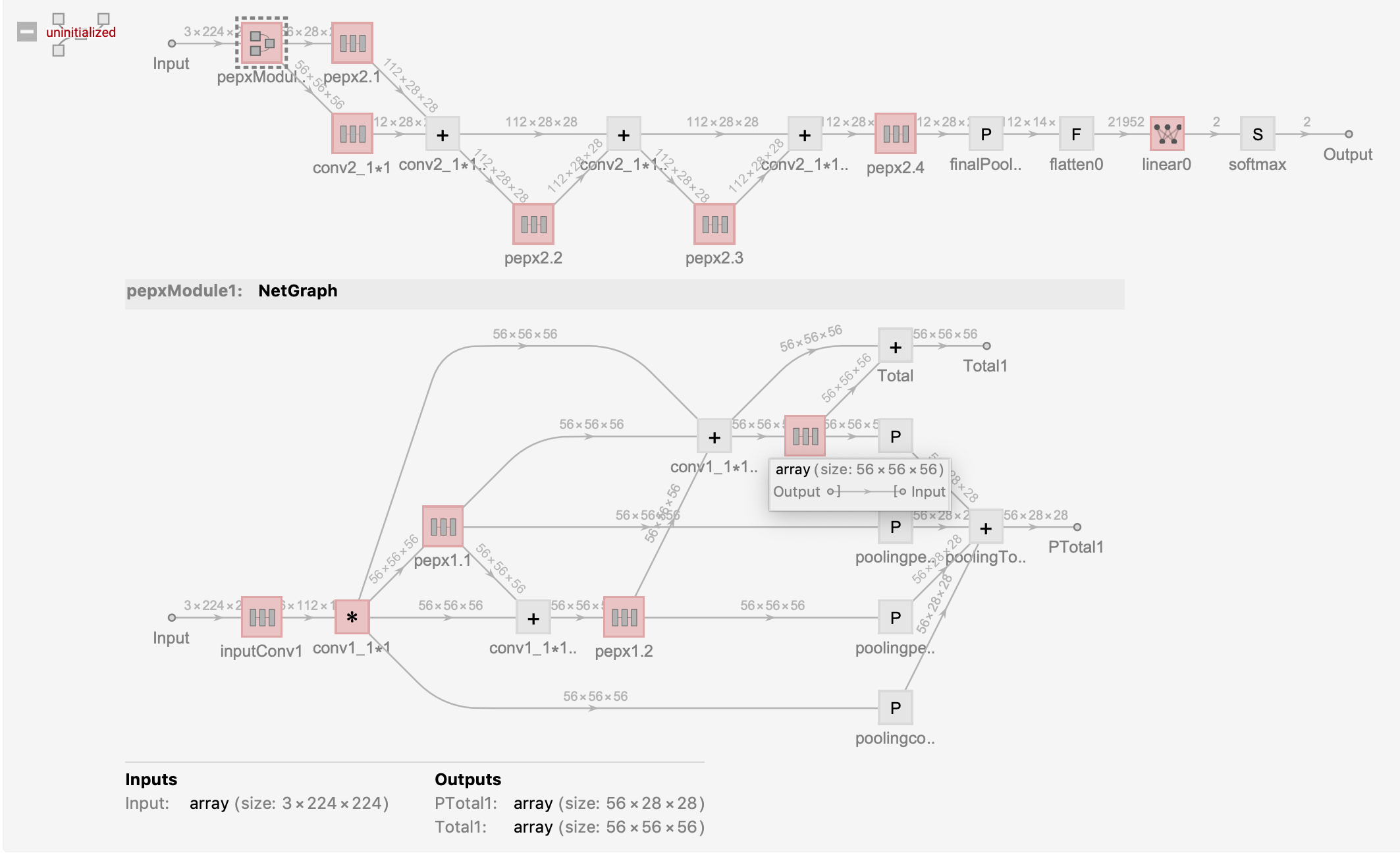
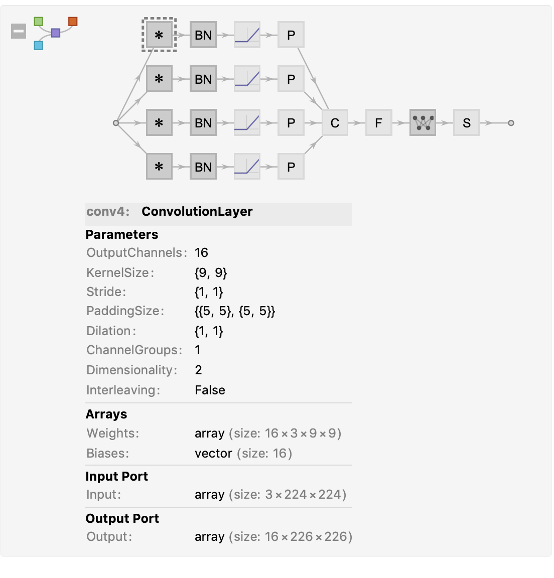
The above test architecture is a part of the computational diagram for Covid-Net’s PEPX{1.1,1.2,1.3}, Conv1_11, Conv2_11, PEPX{2.1,2.2,2.3,2.4}.
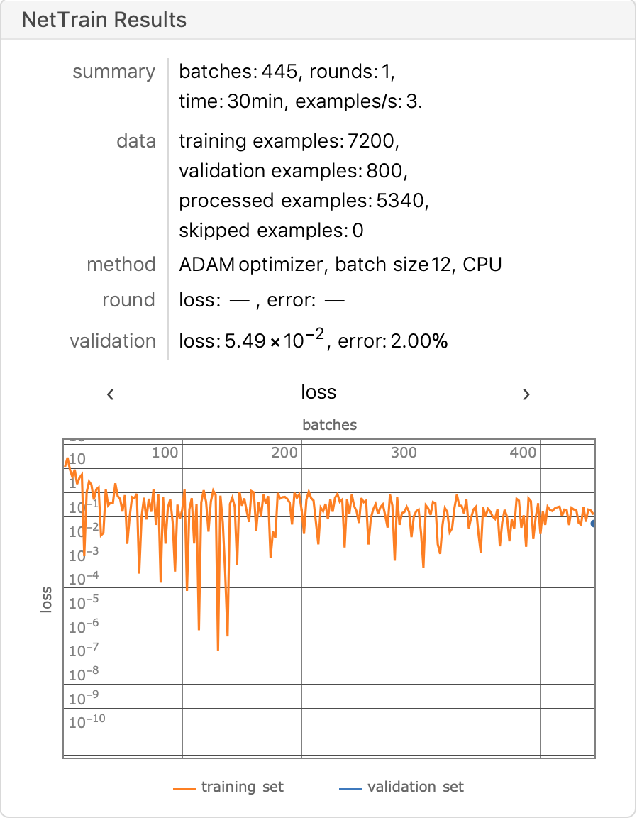
We use this network to train catVSdog and get the training results as follows:
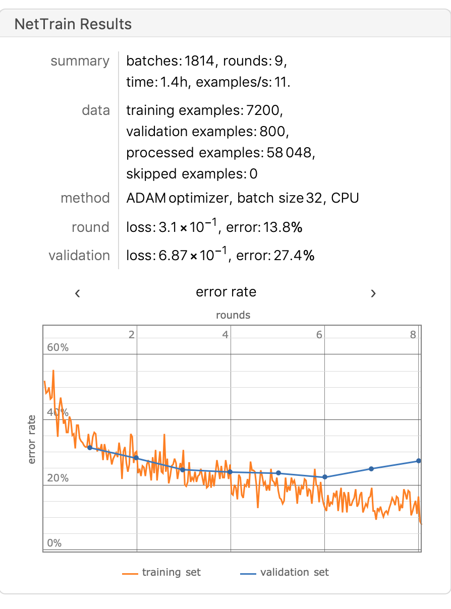
The accuracy on the test set is 75.4%, and in the figure we can see that the model is overfitted starting from the sixth round of training.
Covid-Net uses a 11 convolutional kernel. The features of using a 11 convolutional kernel can be found in the following two articles:
-
[2019-10-31-convolutional-layer-convolution-kernel](https://www.sicara.ai/blog/2019-10-31-convolutional-layer-convolution- kernel)
-
[introduction-to-1x1-convolutions-to-reduce-the-complexity-of-convolutional-neural-networks](https://machinelearningmastery.com /introduction-to-1x1x1-convolutions-to-reduce-the-complexity-of-convolutional-neural-networks/)
1 * 1 Convolution kernels can be used to increase and decrease the number of features, for example, the input dimension is (64,224,224), there are 64 feature channels, the height and width are 224,224, and after processing by the convolution kernel (32,1,1), we have The dimension of the data remains the same (224,224) which means that we have reduced the dimension of the feature channel without changing the original size of the data.
The complete Covid-Net architecture is described in the Model Building section, and we will now move on to data pre-processing, where we filter and tag X-Ray images collected from the Internet.
Data preprocessing
Creating Covidx Data Sets
Build Net Model
Mathematica Code:
pepxModel[inChannel_, outChannel_] := Module[{model}, model = NetChain[
{ConvolutionLayer[Floor[inChannel/2], {1, 1}],
BatchNormalizationLayer[],
Ramp,
ConvolutionLayer[IntegerPart[3*inChannel/4], {1, 1}],
BatchNormalizationLayer[],
Ramp,
ConvolutionLayer[IntegerPart[3*inChannel/4], {3, 3},
PaddingSize -> {1, 1}],
BatchNormalizationLayer[],
Ramp,
ConvolutionLayer[Floor[inChannel/2], {1, 1}],
ConvolutionLayer[outChannel, {1, 1}],
BatchNormalizationLayer[]}];
model]
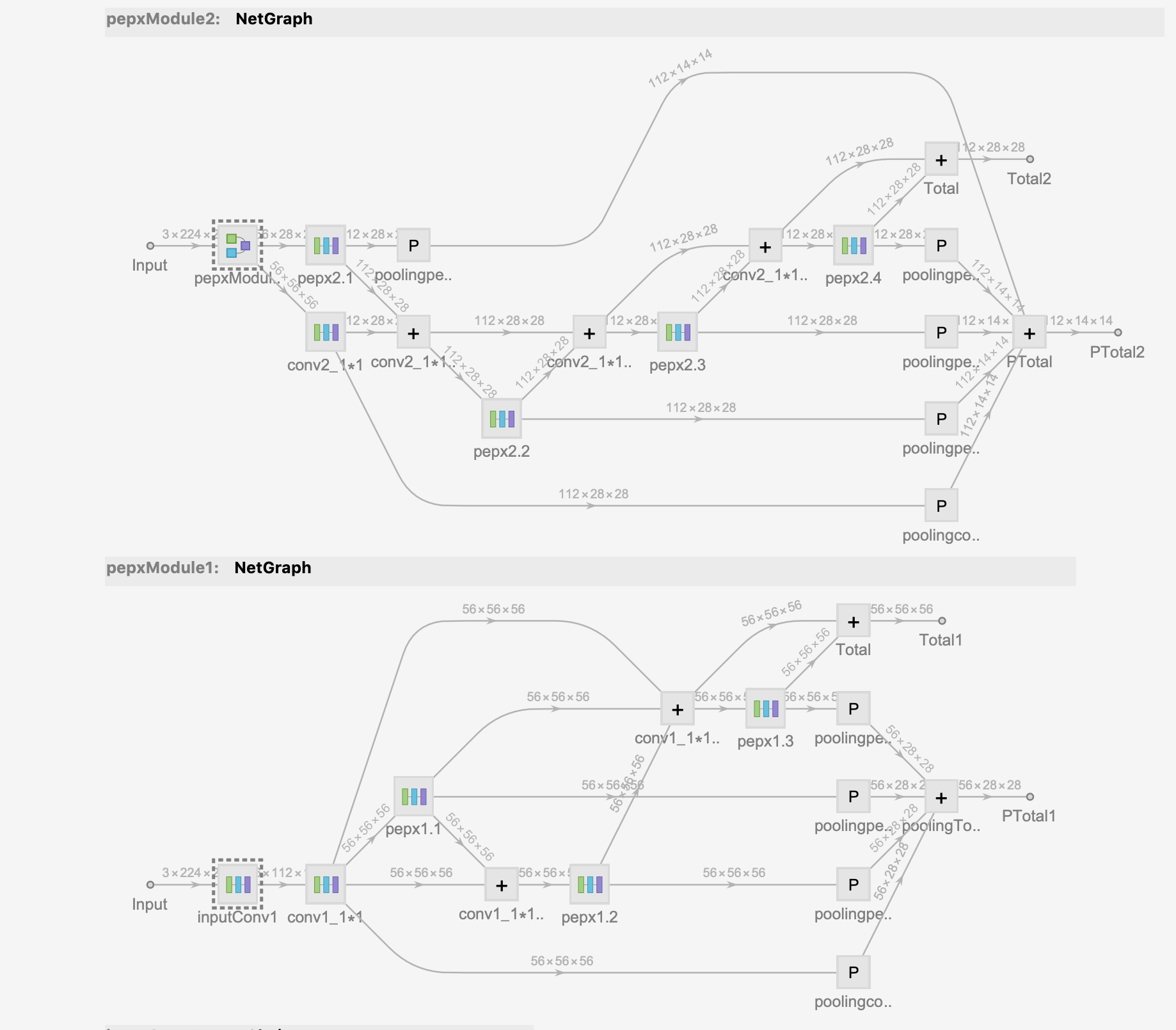
pepxModule1 := NetGraph[<|
"inputConv1" -> NetChain[{
ConvolutionLayer[56, {7, 7}, "Stride" -> {2, 2},
PaddingSize -> {3, 3}],
BatchNormalizationLayer[],
Ramp,
PoolingLayer[{3, 3}, PaddingSize -> {1, 1}]}],
(* block 1 *)
"pepx1.1" -> pepxModel[56, 56],
"pepx1.2" -> pepxModel[56, 56],
"pepx1.3" -> pepxModel[56, 56],
"conv1_1*1" ->
NetChain[{ConvolutionLayer[56, {1, 1}, "Stride" -> {2, 2}],
BatchNormalizationLayer[]}],
"conv1_1*1+pepx1.1" -> TotalLayer[],
"conv1_1*1+pepx1.{1,2}" -> TotalLayer[],
"Total" -> TotalLayer[],
"poolingpepx1.1" -> PoolingLayer[2, 2],
"poolingpepx1.2" -> PoolingLayer[2, 2],
"poolingpepx1.3" -> PoolingLayer[2, 2],
"poolingconv1_1*1" -> PoolingLayer[2, 2],
"poolingTotal" -> TotalLayer[]
|>,
{
"inputConv1" -> "conv1_1*1" -> "pepx1.1" ,
{"pepx1.1", "conv1_1*1"} -> "conv1_1*1+pepx1.1" -> "pepx1.2",
{"pepx1.1", "conv1_1*1", "pepx1.2"} ->
"conv1_1*1+pepx1.{1,2}" -> "pepx1.3",
{"conv1_1*1+pepx1.{1,2}", "pepx1.3"} ->
"Total" -> NetPort["Total1"],
{"pepx1.1" -> "poolingpepx1.1", "pepx1.2" -> "poolingpepx1.2",
"pepx1.3" -> "poolingpepx1.3",
"conv1_1*1" -> "poolingconv1_1*1"} ->
"poolingTotal" -> NetPort["PTotal1"]
}]
pepxModule2 := NetGraph[<|
"pepxModule1" -> pepxModule1,
"pepx2.1" -> pepxModel[56, 112],
"pepx2.2" -> pepxModel[112, 112],
"pepx2.3" -> pepxModel[112, 112],
"pepx2.4" -> pepxModel[112, 112],
"conv2_1*1" -> NetChain[{
ConvolutionLayer[112, {1, 1}],
BatchNormalizationLayer[],
Ramp,
PoolingLayer[2, 2]}],
"conv2_1*1+pepx2.1" -> TotalLayer[],
"conv2_1*1+pepx2.{1,2}" -> TotalLayer[],
"conv2_1*1+pepx2.{1,2,3}" -> TotalLayer[],
"Total" -> TotalLayer[],
"PTotal" -> TotalLayer[],
"poolingpepx2.1" -> PoolingLayer[2, 2],
"poolingpepx2.2" -> PoolingLayer[2, 2],
"poolingpepx2.3" -> PoolingLayer[2, 2],
"poolingpepx2.4" -> PoolingLayer[2, 2],
"poolingconv2_1*1" -> PoolingLayer[2, 2]
|>,
{
NetPort["pepxModule1", "Total1"] -> "conv2_1*1",
NetPort["pepxModule1", "PTotal1"] -> "pepx2.1",
{"conv2_1*1", "pepx2.1"} -> "conv2_1*1+pepx2.1" -> "pepx2.2",
{"conv2_1*1+pepx2.1", "pepx2.2"} ->
"conv2_1*1+pepx2.{1,2}" -> "pepx2.3",
{"conv2_1*1+pepx2.{1,2}", "pepx2.3"} ->
"conv2_1*1+pepx2.{1,2,3}" -> "pepx2.4" ,
{"conv2_1*1+pepx2.{1,2,3}", "pepx2.4"} ->
"Total" -> NetPort["Total2"],
{"pepx2.1" -> "poolingpepx2.1", "pepx2.2" -> "poolingpepx2.2",
"pepx2.3" -> "poolingpepx2.3", "pepx2.4" -> "poolingpepx2.4",
"conv2_1*1" -> "poolingconv2_1*1"} ->
"PTotal" -> NetPort["PTotal2"]
}]
pepxModule3 := NetGraph[<|
"pepxModule2" -> pepxModule2,
"conv3_1*1" -> NetChain[{
ConvolutionLayer[224, {1, 1}],
BatchNormalizationLayer[],
Ramp,
PoolingLayer[2, 2]}],
"pepx3.1" -> pepxModel[112, 224],
"pepx3.2" -> pepxModel[224, 224],
"pepx3.3" -> pepxModel[224, 224],
"pepx3.4" -> pepxModel[224, 224],
"pepx3.5" -> pepxModel[224, 224],
"pepx3.6" -> pepxModel[224, 224],
"conv3_1*1+pepx3.1" -> TotalLayer[],
"conv3_1*1+pepx3{1,2}" -> TotalLayer[],
"conv3_1*1+pepx3{1,2,3}" -> TotalLayer[],
"conv3_1*1+pepx3{1,2,3,4}" -> TotalLayer[],
"conv3_1*1+pepx3{1,2,3,4,5}" -> TotalLayer[],
"Total" -> TotalLayer[],
"PTotal" -> TotalLayer[],
"poolingpepx3.1" -> PoolingLayer[2, 2],
"poolingpepx3.2" -> PoolingLayer[2, 2],
"poolingpepx3.3" -> PoolingLayer[2, 2],
"poolingpepx3.4" -> PoolingLayer[2, 2],
"poolingpepx3.5" -> PoolingLayer[2, 2],
"poolingpepx3.6" -> PoolingLayer[2, 2],
"poolingconv3_1*1" -> PoolingLayer[2, 2]
|>,
{
NetPort["pepxModule2", "Total2"] -> "conv3_1*1",
NetPort["pepxModule2", "PTotal2"] -> "pepx3.1",
{"pepx3.1", "conv3_1*1"} -> "conv3_1*1+pepx3.1" -> "pepx3.2",
{"conv3_1*1+pepx3.1", "pepx3.2"} ->
"conv3_1*1+pepx3{1,2}" -> "pepx3.3",
{"conv3_1*1+pepx3{1,2}" , "pepx3.3"} ->
"conv3_1*1+pepx3{1,2,3}" -> "pepx3.4",
{"conv3_1*1+pepx3{1,2,3}", "pepx3.4"} ->
"conv3_1*1+pepx3{1,2,3,4}" -> "pepx3.5",
{ "conv3_1*1+pepx3{1,2,3,4}" , "pepx3.5"} ->
"conv3_1*1+pepx3{1,2,3,4,5}" -> "pepx3.6",
{"conv3_1*1+pepx3{1,2,3,4,5}", "pepx3.6"} ->
"Total" -> NetPort["Total3"],
{"pepx3.1" -> "poolingpepx3.1", "pepx3.2" -> "poolingpepx3.2",
"pepx3.3" -> "poolingpepx3.3", "pepx3.4" -> "poolingpepx3.4",
"pepx3.5" -> "poolingpepx3.5", "pepx3.6" -> "poolingpepx3.6",
"conv3_1*1" -> "poolingconv3_1*1"} ->
"PTotal" -> NetPort["PTotal3"]
}]
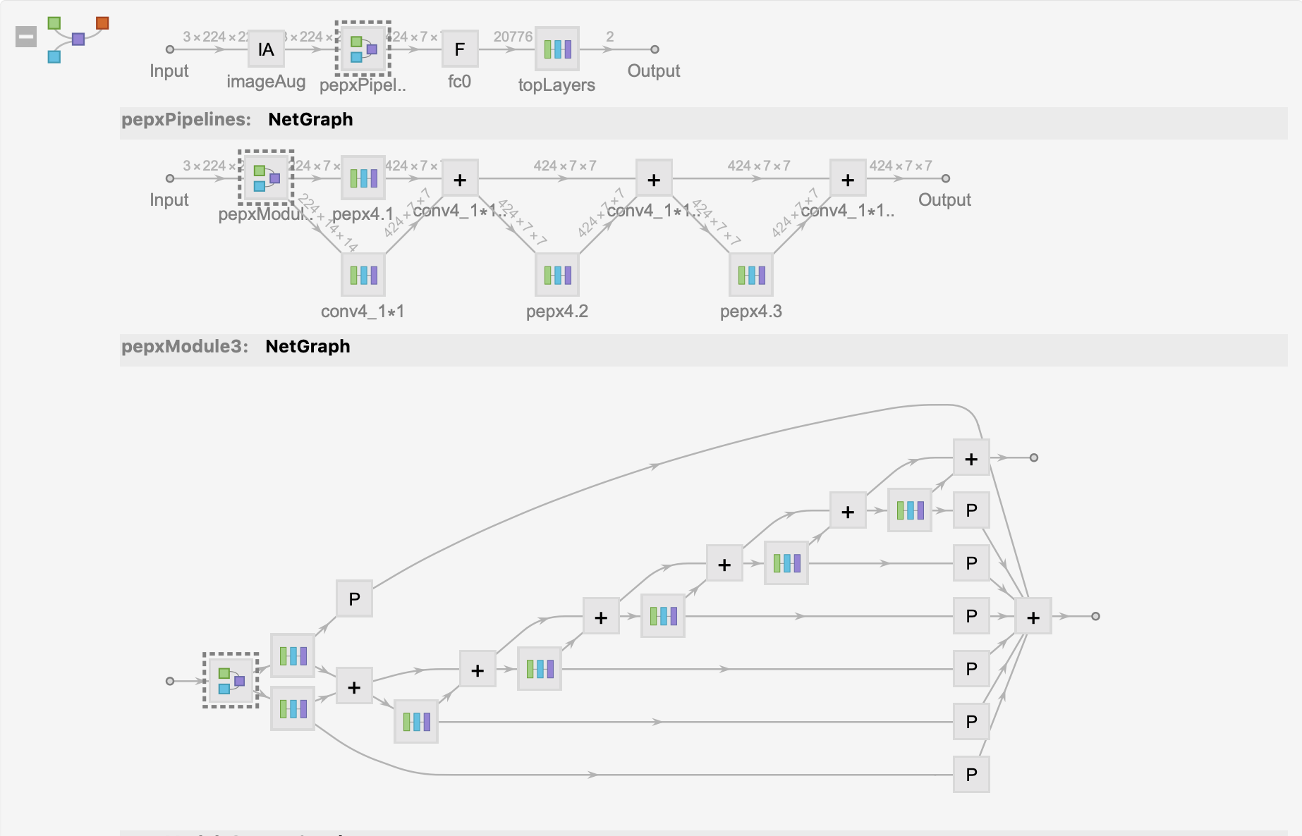
pepxModule4 := NetGraph[<|
"pepxModule3" -> pepxModule3,
"conv4_1*1" -> NetChain[{
ConvolutionLayer[424, {1, 1}],
BatchNormalizationLayer[],
Ramp,
PoolingLayer[2, 2]}],
"pepx4.1" -> pepxModel[224, 424],
"pepx4.2" -> pepxModel[424, 424],
"pepx4.3" -> pepxModel[424, 424],
"conv4_1*1+pepx4.1" -> TotalLayer[],
"conv4_1*1+pepx4.{1,2}" -> TotalLayer[],
"conv4_1*1+pepx4.{1,2,3}" -> TotalLayer[]
|>,
{
NetPort["pepxModule3", "Total3"] -> "conv4_1*1",
NetPort["pepxModule3", "PTotal3"] -> "pepx4.1",
{"pepx4.1", "conv4_1*1"} -> "conv4_1*1+pepx4.1" -> "pepx4.2",
{"conv4_1*1+pepx4.1", "pepx4.2"} ->
"conv4_1*1+pepx4.{1,2}" -> "pepx4.3",
{"conv4_1*1+pepx4.{1,2}", "pepx4.3"} -> "conv4_1*1+pepx4.{1,2,3}"
}]
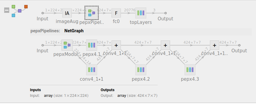
covidNet =
NetInitialize[
NetGraph[<|
"imageAug" -> ImageAugmentationLayer[{224, 224}],
"pepxPipelines" -> pepxModule4,
"fc0" -> FlattenLayer[],
"topLayers" -> NetChain[{
LinearLayer[1024],
Ramp,
DropoutLayer[],
LinearLayer[256],
Ramp,
LinearLayer[2],
SoftmaxLayer[]}]
|>,
{
"imageAug" -> "pepxPipelines" -> "fc0" -> "topLayers"
},
"Input" -> NetEncoder[{"Image", {224, 224}, ColorSpace -> "RGB"}],
"Output" -> NetDecoder[{"Class", {"cat", "dog"}}]],
Method -> {"Xavier", "Distribution" -> "Uniform"}]
The model architecture is shown below:
Finally, training the model on the CatDog dataset with your own laptop after 🔟 rounds yields about 80% accuracy.
Finally, we trained the model on a workstation, and the DogCat dataset was increased to 25,000 images to enhance the generalizability of the model, with nearly 92% accuracy after the 🔟 round.
The model was nearly 92% accurate after the training 🔟 round.
Finally, we classify the collected xRay images with labels = {“COVID-19”, “NORMAL”, “PNEUMONIA”}
The datasets are: ieee8023Data,Figure1-COVID-chest-x-ray-dataset,ActualmedDataSets,radiography datasets, the total number of datasets is 3551 xray, of which covide-19 accounts for 763.
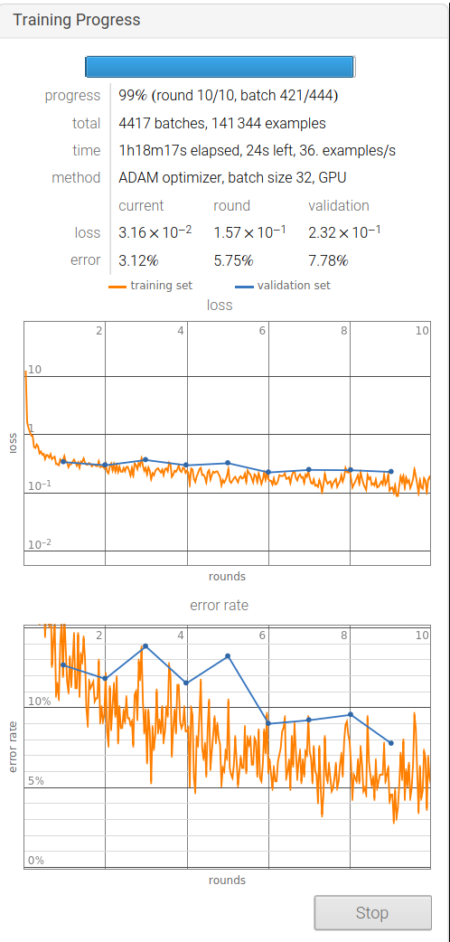
After dividing the datasets into training set and validation set, we start to train the model. 676 pieces of covid-19 in the training set and 87 pieces of covid-19 in the validation set are used.
Training Model
The final model architecture is as follows:
covidNetTrained =
 NetTrain[covidNet, traingDataSets, All, TargetDevice -> "GPU",
  ValidationSet -> validationDataSets,
  TrainingProgressCheckpointing -> {"Directory", dir},
  TrainingProgressReporting -> "Panel", BatchSize -> 32,
  TrainingStoppingCriterion -> <|"Criterion" -> "Loss",
    "Patience" -> 5|>]
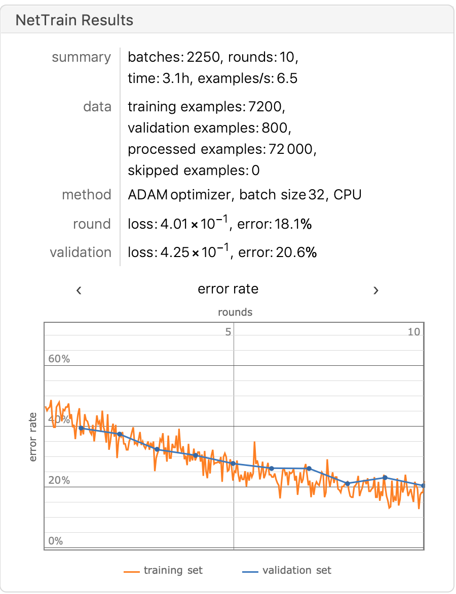
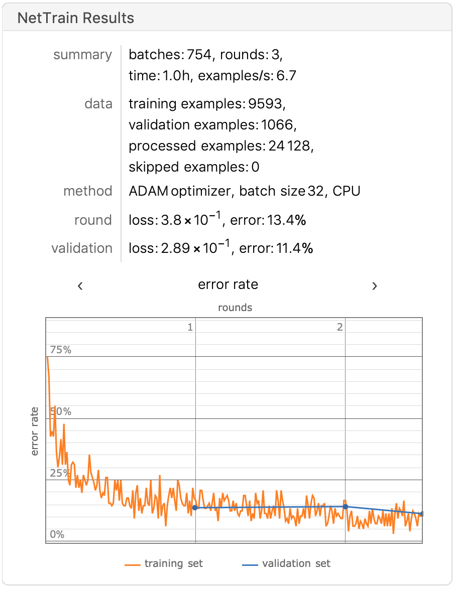
Final Training Results:
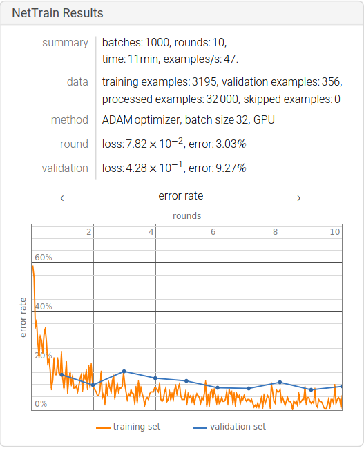
We can find that the accuracy of the model is about 90%. Due to the small size of the data set, there is still a lot of room for improvement of the training results of the model. The transformations can be classified as (Flip, Rotation, Scale, Crop, Translation, Gaussian Noise).
Data Set Enhancement
genDatasets[origindataset_] :=
 Module[{file, label, img, basename, dims},
  file = Keys[origindataset];
  label = Values[origindataset];
  basename = FileBaseName[List @@ file[[1]]];
  If[Not@DirectoryQ[cleandatasetsDir <> label],
   CreateDirectory[cleandatasetsDir <> label]];
  img = Import@file;
  (* rotate *)

  Export[cleandatasetsDir <> label <> "/" <> basename <> "_rotate" <>
    ".png" ,
   ImageRotate[img, RandomReal[] * 2 \[Pi],
    Background -> Transparent]];
  (* reflect *)

  Export[cleandatasetsDir <> label <> "/" <> basename <> "_reflect" <>
    ".png",
   ImageReflect[img, RandomChoice[{Bottom, Top, Left}]]];
  (* crop *)

  Export[cleandatasetsDir <> label <> "/" <> basename <> "_crop" <>
    ".png",
   ImageCrop[
    img, {ImageDimensions[img][[1]] / RandomReal[{1, 1.5}],
     ImageDimensions[img][[2]]/ RandomReal[{1, 1.5}]}]];
  (* blur *)

  Export[cleandatasetsDir <> label <> "/" <> basename <> "_blur" <>
    ".png",
   GaussianFilter[img, RandomInteger[{1, 2}]]];
  (* origin *)

  Export[cleandatasetsDir <> label <> "/" <> basename <> ".png",
   img];
  ]
We need to rotate and reflect the original image to be able to generalize the model better. The generating functions are included in the final code file, using the above functions we crop, rotate and flip the image and process the blurring.
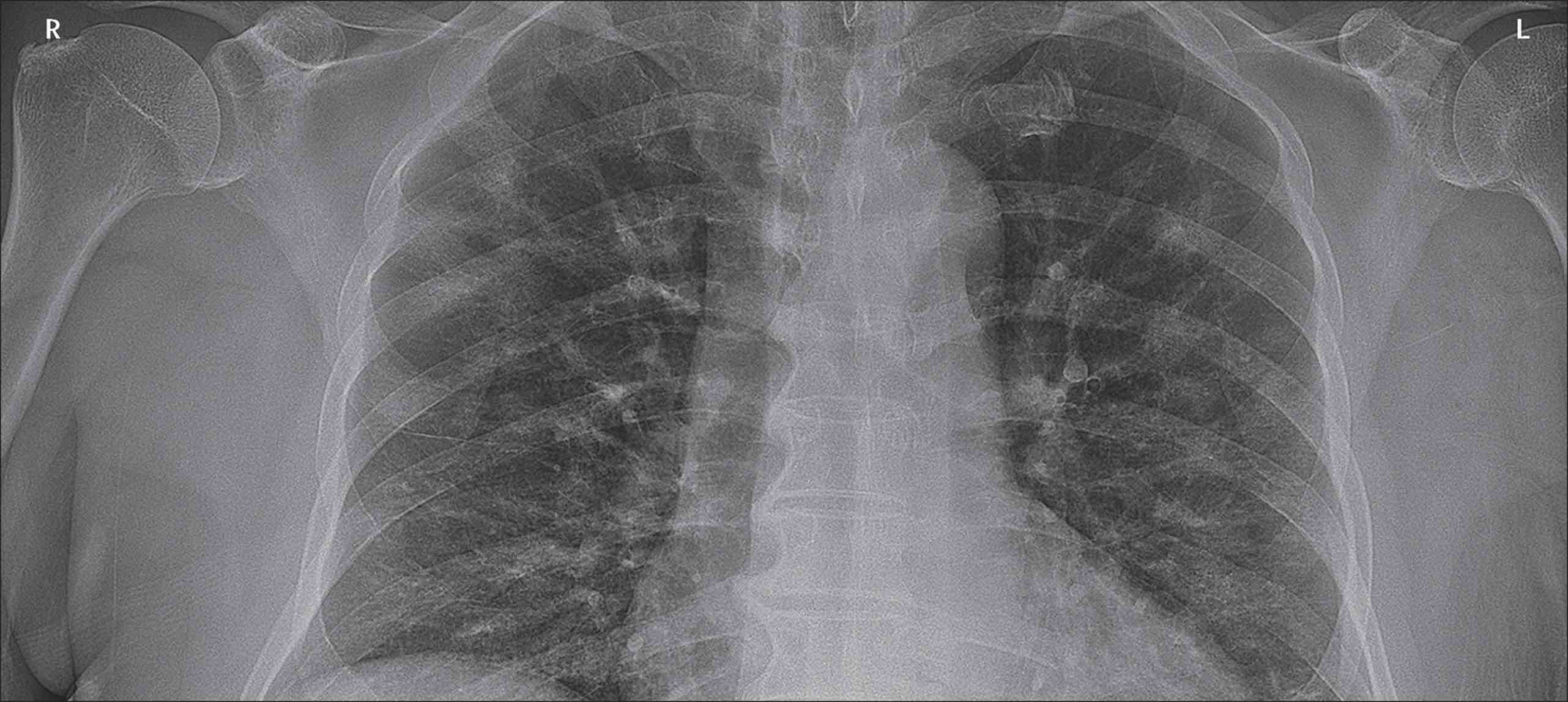
The original image:
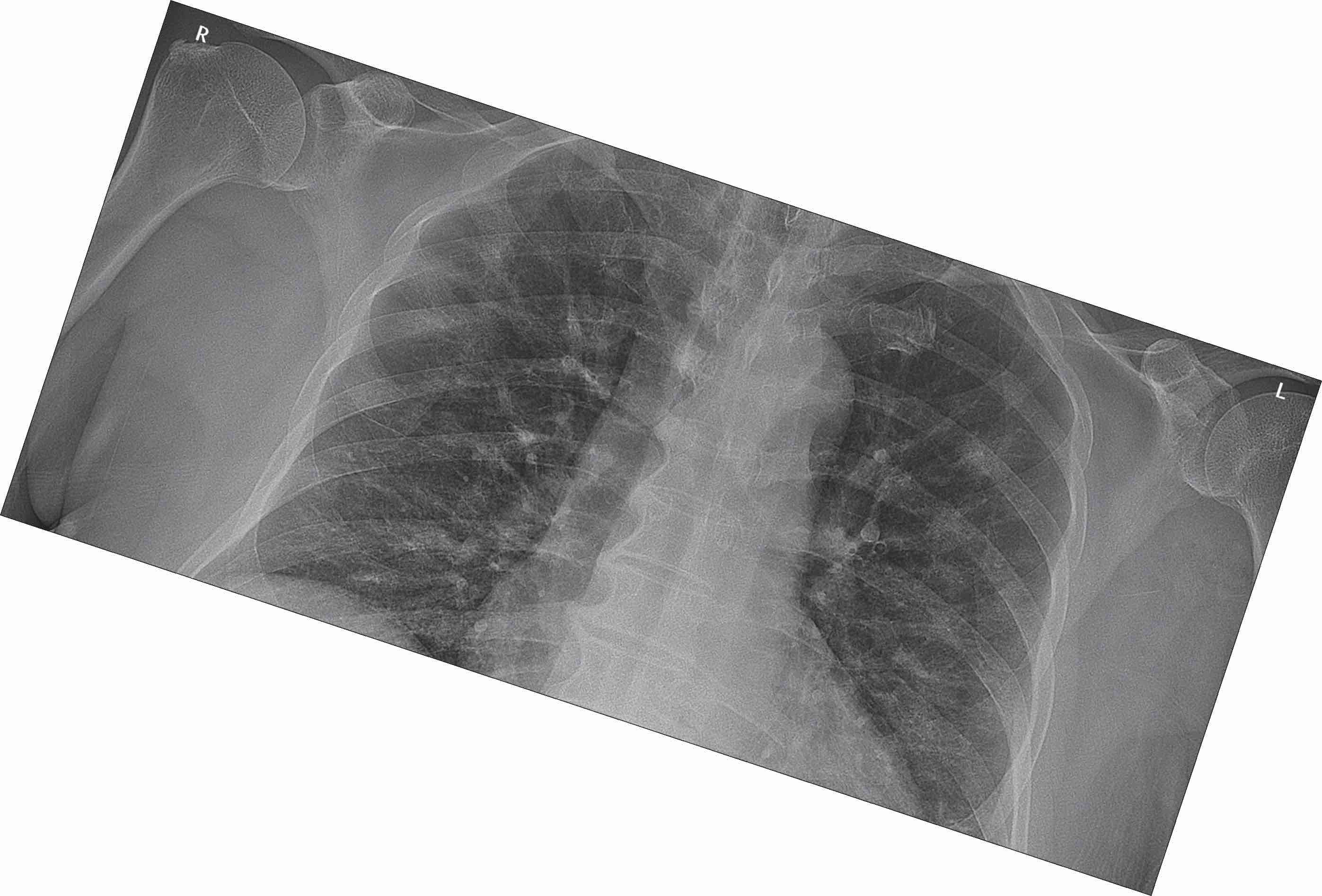
Randomly rotate the image.
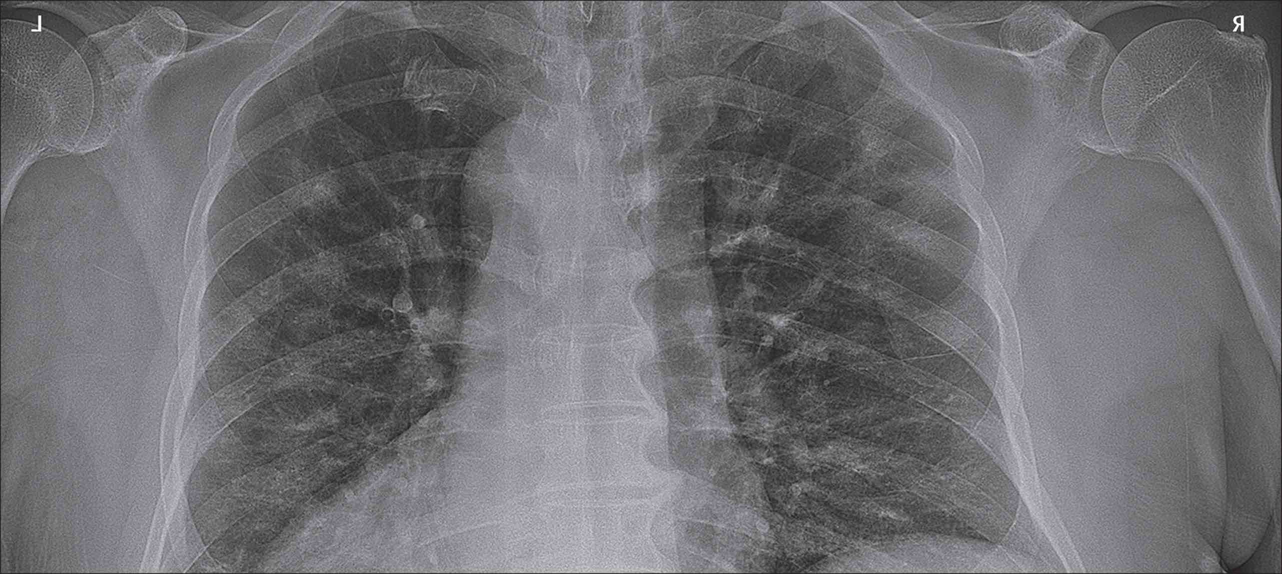
Reflected Images
Finally, merge these generated images into the training and validation set test set.
Test Model
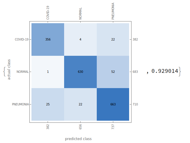
The model is trained on an augmented dataset for a limited duration of one hour:
Accuracy approaching 90%.
Finally, set EPOCHS=10, batch_size=32, and divide the training set:verification set:test set into 8:1:1, and the training results are as follows.
We used the Recall Precision Accuracy F1-Score as a measure of our ability to judge the validity of the model’s prediction of SARS-COV-2, calculated as follows.
TP: True Positive FP: False Positive TN: True Negative FN: False Negative
Recall = TP / (TP + FN)
Precision = TP / (TP + FP)
Accuracy = (TP + TN) / (TP + TN + FP + FN)
F1-Score = 2 * (Recall * Precision) / (Recall + Precision)
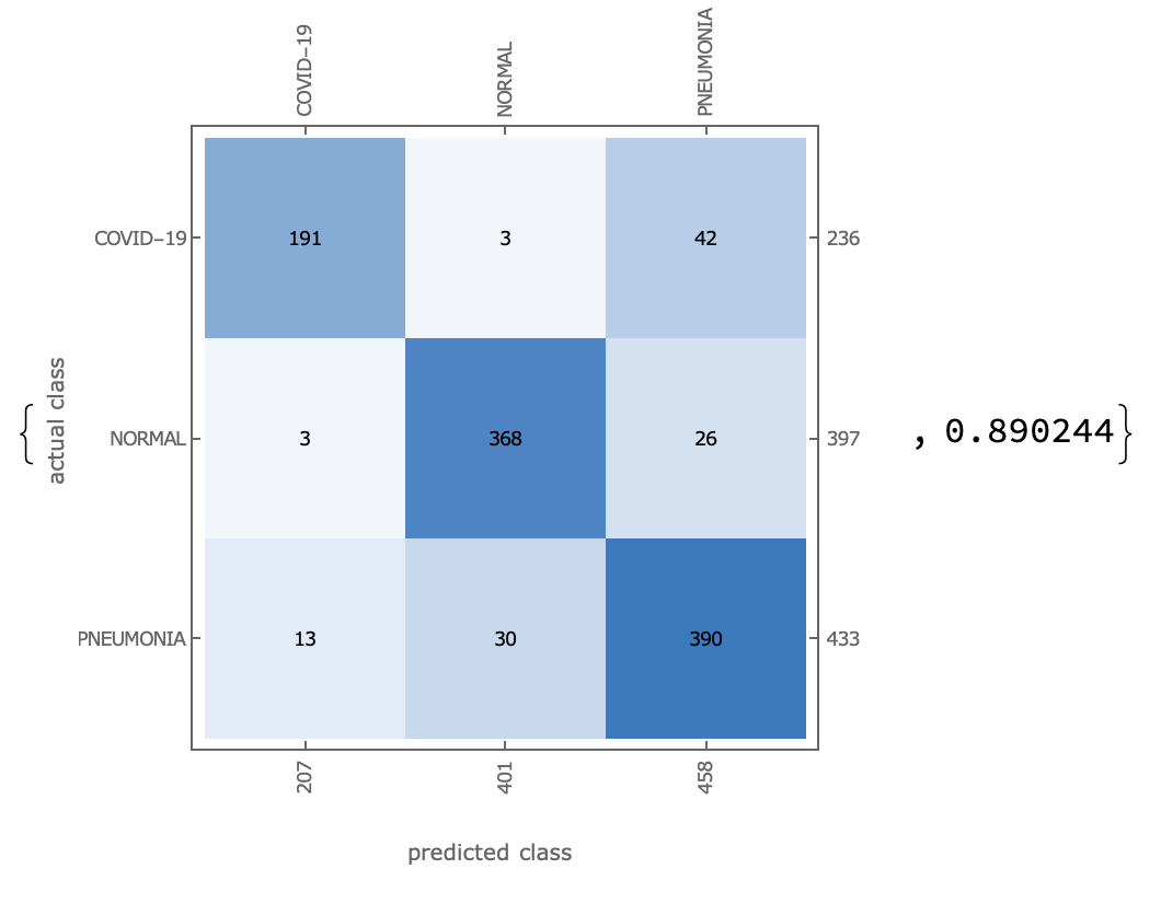
The results are as follows:
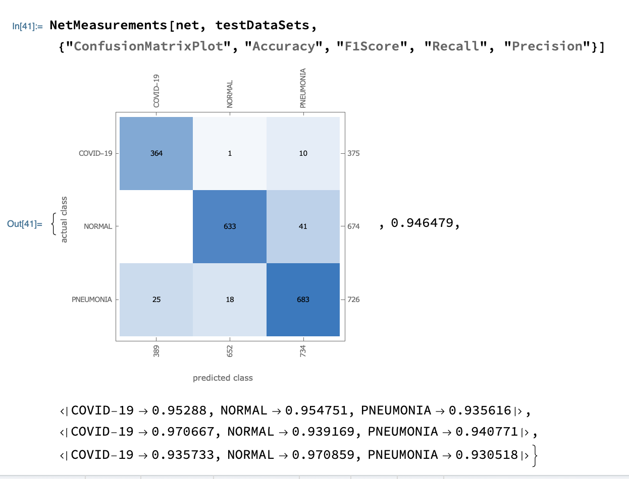
The recall rate for Covid-19 was 97%, meaning that the accuracy of the diagnosis of disease among all Covid-19 patients was 97%.
The accuracy of Covid-19 is 93%, meaning that it can be predicted to be Covid-19 in all samples with 93% accuracy.
The final F1-Score was 95%.
Covid-Net vs. ResNet-50 migration learning
resNet = NetModel["ResNet-50 Trained on ImageNet Competition Data"];
featureNet = NetTake[resNet, {1, -4}];
covidResNet = NetChain[<|
"featuresNet" -> featureNet,
"f0" -> FlattenLayer[],
"linear1" -> LinearLayer[3],
"soft" -> SoftmaxLayer[]|>,
"Input" -> NetEncoder[{"Image", {224, 224}, ColorSpace -> "RGB"}],
"Output" -> NetDecoder[{"Class", labels}]];
dir = CreateDirectory["/Volumes/DataSets/transfermodels"];
covidTrainedNet =
NetTrain[covidResNet, traingDataSets,
ValidationSet -> validationDataSets,
LearningRateMultipliers -> {"featuresNet" -> 0, _ -> 1},
TrainingProgressCheckpointing -> {"Directory", dir},
TrainingStoppingCriterion -> <|"Criterion" -> "Loss",
"Patience" -> 4|>,
BatchSize -> 32]
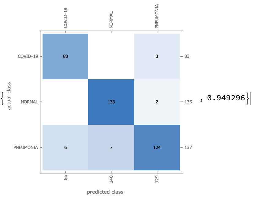
NetMeasurements[covidTrainedNet, validationDataSets, \
{"ConfusionMatrixPlot", "Accuracy"}]
Results of the ResNet model after migration learning.
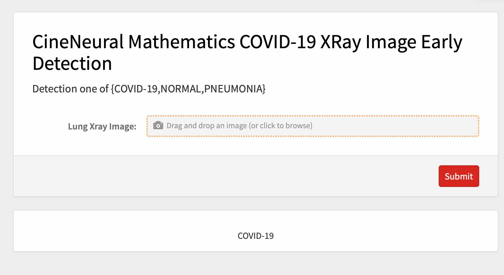
Deployment model
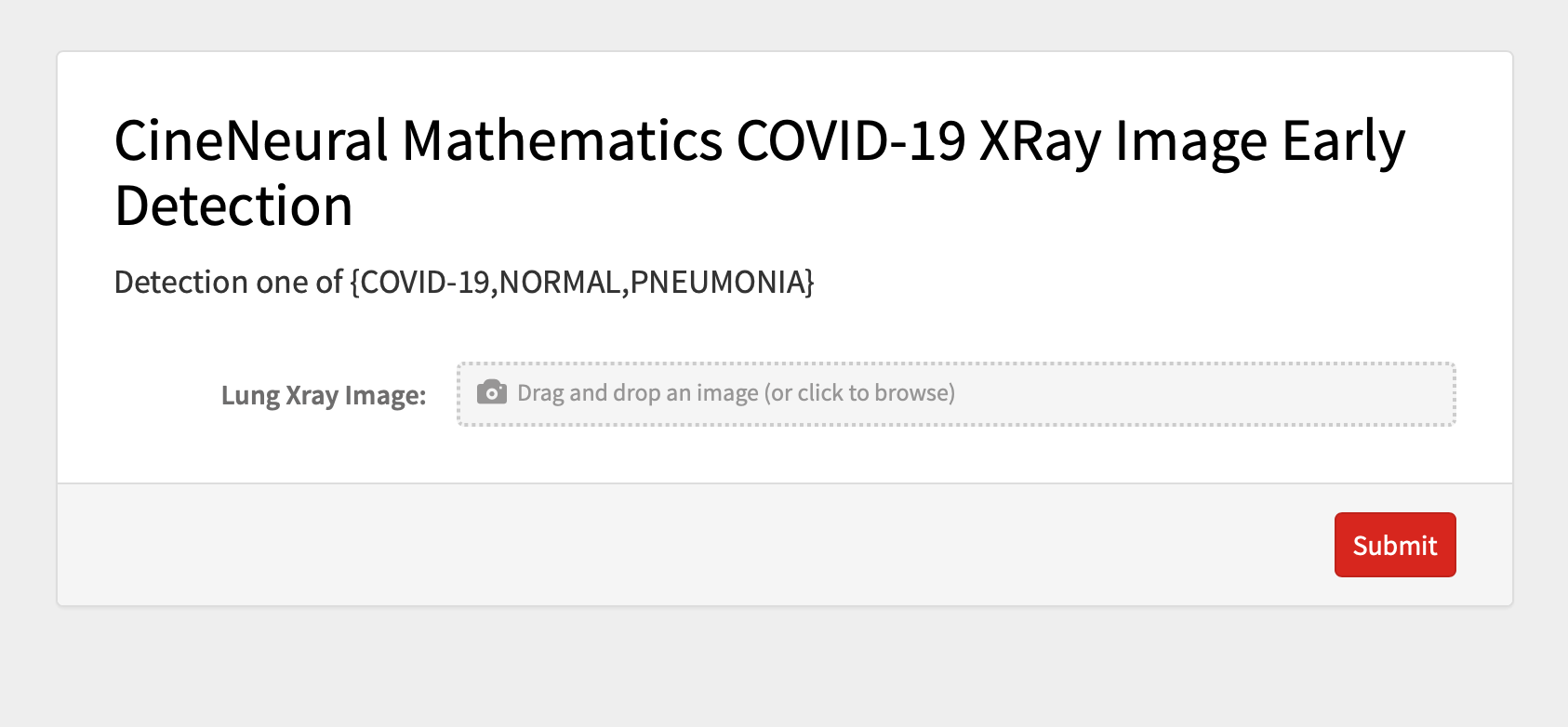
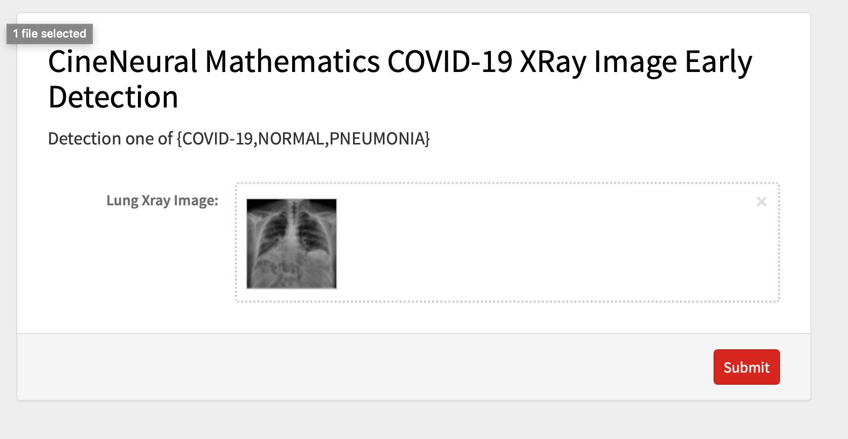
We will be using Wolfram Cloud to deploy our covidResNet and covid-Net.
(* Upload training models to Wolfram Cloud *)
netlink = CloudExport[covidTrainedNet, "MX", Permissions -> "Public"]

(* Deploy pages and processing functions to Cloud *)
CloudDeploy[
 FormPage[{{"image", "Lung Xray Image: "} -> "Image"},
  With[{net = CloudImport@netlink}, net[#image]] &,
  AppearanceRules -> <|

    "Title" ->
     "CineNeural Mathematics COVID-19 XRay Image Early Detection",
    "Description" -> "Detection one of {COVID-19,NORMAL,PNEUMONIA}"|>],
 Permissions -> "Public"]
Page follows:
CineNeural Mathematics COVID-19 XRay Image Early Detection
Deploy model to local Coral dev Board
Deploying models locally is the future of deep learning, and in this section we will combine Tensorflow and Mathematica to run the trained models on the google coral dev board.